Force Fields and Interactions
Overview
Teaching: 30 min
Exercises: 0 minQuestions
What is Molecular Dynamics and how can I benefit from using it?
What is a force field?
What mathematical energy terms are used in biomolecular force fields?
Objectives
Understand strengths and weaknesses of MD simulations
Understand how the interactions between particles in a molecular dynamics simulation are modeled
Introduction
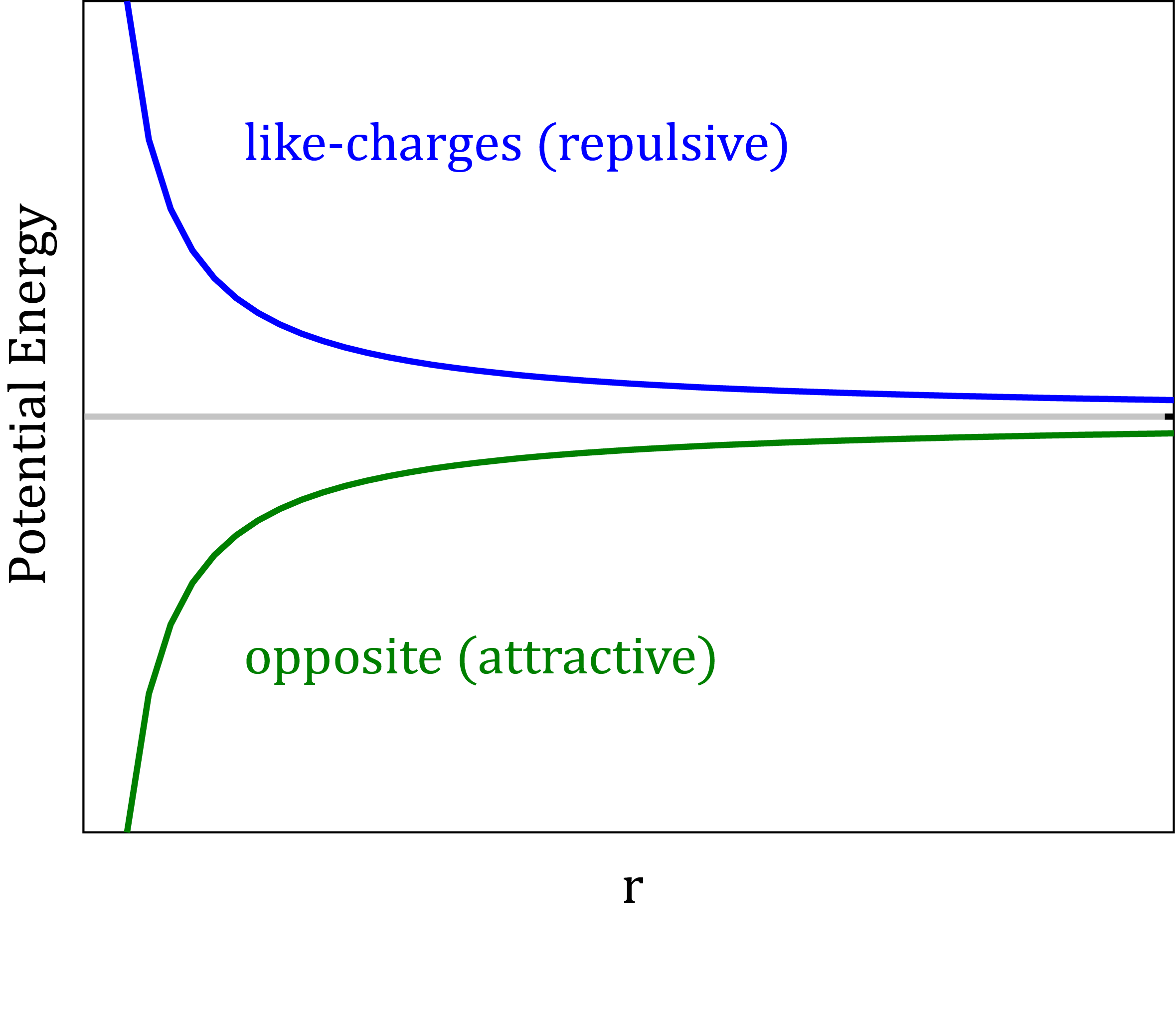
Atoms and molecules, the building blocks of matter, interact with each other. They are attracted at long distances, but at short distances the interactions become strongly repulsive. As a matter of fact, there is no need to look for a proof that such interactions exist. Every day, we observe indirect results of these interactions with our own eyes. For example, because of the attraction between water molecules, they stick together to form drops, which then rain down to fill rivers. On the other hand, due to the strong repulsion, one liter of the same water always weighs about 1 kg, regardless of how much pressure we use to compress it.
Nowadays, molecular modeling is done by analyzing dynamic structural models in computers. Historically, the modeling of molecules started long before the invention of computers. In the mid-1800’s structural models were suggested for molecules to explain their chemical and physical properties. First attempts at modeling interacting molecules were made by van der Waals in his pioneering work “About the continuity of the gas and liquid state” published in 1873. A simple equation representing molecules as spheres that are attracted to each other enabled him to predict the transition from gas to liquid. Modern molecular modeling and simulation still rely on many of the concepts developed over a century ago. Recently, MD simulations have been vastly improved in size and length. With longer simulations, we are able to study a broader range of problems under a wider range of conditions.
- Atoms and molecules interact with each other.
- We carry out molecular modeling by following and analyzing dynamic structural models in computers.
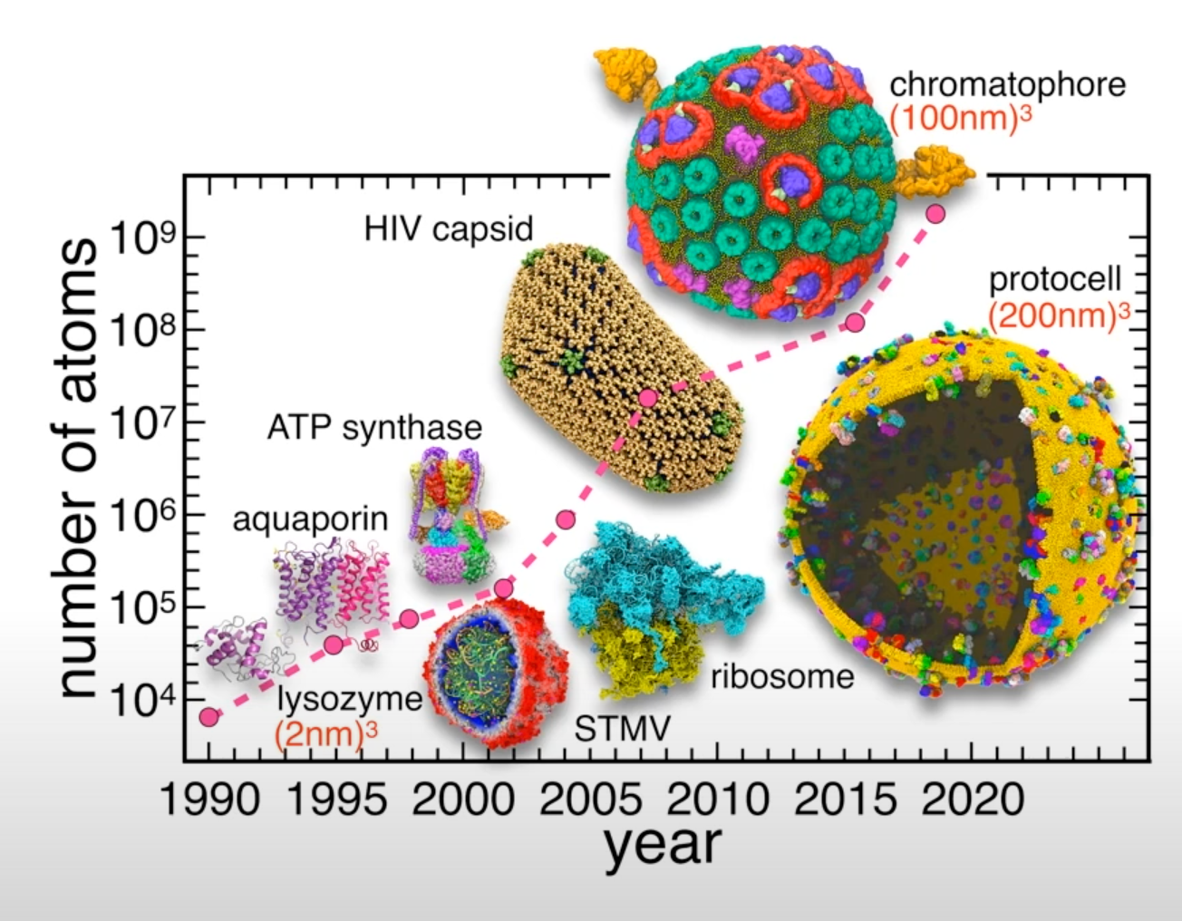 Figure from: AI-Driven Multiscale Simulations Illuminate Mechanisms of SARS-CoV-2 Spike Dynamics
- The size and the length of MD simulations has been recently vastly improved.
- Longer and larger simulations allow us to tackle wider range of problems under a wide variety of conditions.
Recent example - simulation of the whole SARS-CoV-2 virion
One of the recent examples is simulation of the whole SARS-CoV-2 virion. The goal of this work was to understand how this virus infects cells. As a result of MD simulations, conformational transitions of the spike protein as well as its interactions with ACE2 receptors were identified. According to the simulation, the receptor binding domain of the spike protein, which is concealed from antibodies by polysaccharides, undergoes conformational transitions that allow it to emerge from the glycan shield and bind to the angiotensin-converting enzyme (ACE2) receptor in host cells.
The virion model included 305 million atoms, it had a lipid envelope of 75 nm in diameter with a full virion diameter of 120 nm. The multiscale simulations were performed using a combination of NAMD, VMD, AMBER. State-of-the-art methods such as the Weighted Ensemble Simulation Toolkit and ML were used. The whole system was simulated on the Summit supercomputer at Oak Ridge National Laboratory for a total time of 84 ns using NAMD. In addition a weighted ensemble of a smaller spike protein systems was simulated using GPU accelerated AMBER software.
This is one of the first works to explore how machine learning can be applied to MD studies. Using a machine learning algorithm trained on thousands of MD trajectory examples, conformational sampling was intelligently accelerated. As a result of applying machine learning techniques, it was possible to identify pathways of conformational transitions between active and inactive states of spike proteins.
- System size: 304,780,149 atoms, 350 Å × 350 Å lipid bilayer, simulation time 84 ns
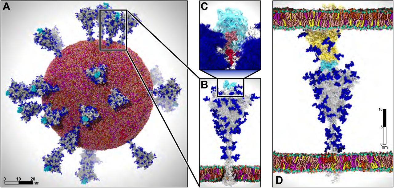 Figure from AI-Driven Multiscale Simulations Illuminate Mechanisms of SARS-CoV-2 Spike Dynamics
- Showed that spike glycans can modulate the infectivity of the virus.
- Characterized interactions between the spike and the human ACE2 receptor.
- Used ML to identify conformational transitions between states and accelerate conformational sampling.
Goals
In this workshop, you will learn about molecular dynamics simulations and how to use different molecular dynamics simulation packages and utilities, such as NAMD, VMD, and AMBER. We will show you how to use Digital Research Alliance of Canada (Alliance) clusters for all steps of preparing the system, performing MD and analyzing the data. The emphasis will be on reproducibility and automation through scripting and batch processing.
- Introduce you to the method of molecular dynamics simulations.
- Guide you to using various molecular dynamics simulation packages and utilities.
- Teach how to use Digital Research Alliance of Canada (Alliance) clusters for system preparation, simulation and trajectory analysis.
The goal of this first lesson is to provide an overview of the theoretical foundation of molecular dynamics. As a result of this lesson, you will gain a deeper understanding of how particle interactions are modeled and how molecular dynamics are simulated.
The focus will be on reproducibility and automation by introducing scripting and batch processing.
The theory behind the method of MD.
Force Fields
The development of molecular dynamics was largely motivated by the desire to understand complex biological phenomena at the molecular level. To gain a deeper understanding of such processes, it was necessary to simulate large systems over a long period of time.
While the physical background of intermolecular interactions is known, there is a very complex mixture of quantum mechanical forces acting at a close distance. The forces between atoms and molecules arise from dynamic interactions between numerous electrons orbiting atoms. Since the interactions between electron clouds are so complex, they cannot be described analytically, nor can they be calculated numerically fast enough to enable a dynamic simulation on a relevant scale.
In order for molecular dynamics simulations to be feasible, it was necessary to be able to evaluate molecular interactions very quickly. To achieve this goal molecular interactions in molecular dynamics are approximated with a simple empirical potential energy function.
- Understanding complex biological phenomena requires simulations of large systems for a long time windows.
- The forces acting between atoms and molecules are very complex.
- Very fast method of evaluations molecular interactions is needed to achieve these goals.
Interactions are approximated with a simple empirical potential energy function.
The potential energy function U is a cornerstone of the MD simulations because it allows calculating forces. A force on an object is equal to the negative of the derivative of the potential energy function:
$\vec{F}=-\nabla{U}(\vec{r})$
Once we know forces acting on an object we can calculate how its position changes in time. To advance a simulation in time molecular dynamics applies classical Newton’s equation of motion stating that the rate of change of momentum \(\vec{p}\) of an object equals the force \(\vec{F}\) acting on it:
$ \vec{F}=\frac{d\vec{p}}{dt} $
To summarize, if we are able to determine a system’s potential energy, we can also determine the forces acting between the particles as well as how their positions change over time. In other words, we need to know the interaction potential for the particles in the system to calculate forces acting on atoms and advance a simulation.
- The potential energy function allows calculating forces: $ \vec{F}=-\nabla{U}(\vec{r}) $
- With the knowledge of the forces acting on an object, we can calculate how the position of that object changes over time: $ \vec{F}=\frac{d\vec{p}}{dt} $.
- Advance system with very small time steps assuming the velocities don’t change.
Let’s examine a typical workflow for simulations of molecular dynamics.
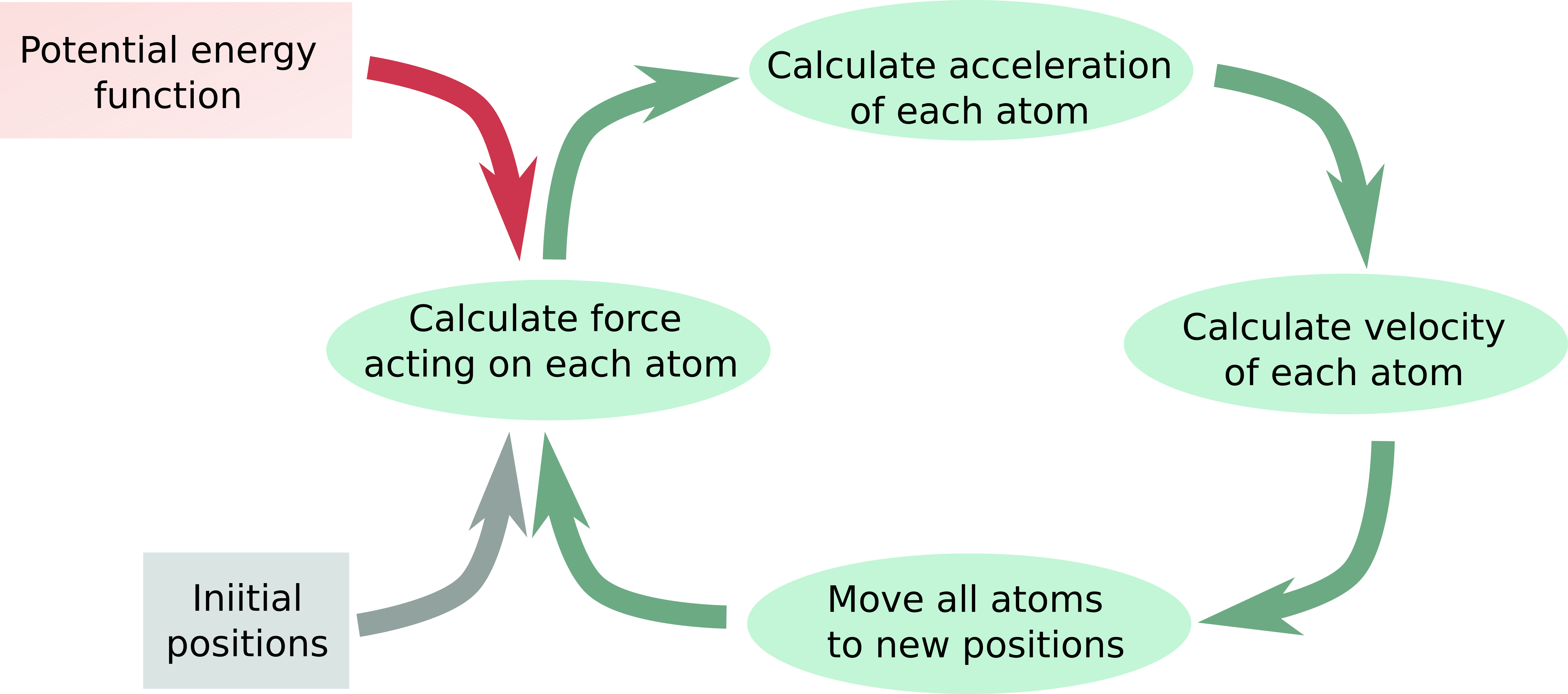 Flow diagram of MD simulation
A force field is a set of empirical energy functions and parameters used to calculate the potential energy U as a function of the molecular coordinates.
Molecular dynamics programs use force fields to run simulations. A force field (FF) is a set of empirical energy functions and parameters allowing to calculate the potential energy U of a system of atoms and/or molecules as a function of the molecular coordinates. Classical molecular mechanics potential energy function used in MD simulations is an empirical function composed of non-bonded and bonded interactions:
- Potential energy function used in MD simulations is composed of non-bonded and bonded interactions:
$U(\vec{r})=\sum{U_{bonded}}(\vec{r})+\sum{U_{non-bonded}}(\vec{r})$
Typically MD simulations are limited to evaluating only interactions between pairs of atoms. In this approximation force fields are based on two-body potentials, and the energy of the whole system is described by the 2-dimensional force matrix of the pairwise interactions.
- Only pairwise interactions are considered.
Classification of force fields.
For convenience force fields can be divided into 3 general classes based on how complex they are.
Class 1 force fields.
In the class 1 force field dynamics of bond stretching and angle bending are described by simple harmonic motion, i.e. the magnitude of restoring force is assumed to be proportional to the displacement from the equilibrium position. As the energy of a harmonic oscillator is proportional to the square of the displacement, this approximation is called quadratic. In general, bond stretching and angle bending are close to harmonic only near the equilibrium. Higher-order anharmonic energy terms are required for a more accurate description of molecular motions. In the class 1 force field force matrix is diagonal because correlations between bond stretching and angle bending are omitted.
- Dynamics of bond stretching and angle bending is described by simple harmonic motion (quadratic approximation)
- Correlations between bond stretching and angle bending are omitted.
Examples: AMBER, CHARMM, GROMOS, OPLS
Class 2 force fields.
Class 2 force fields add anharmonic cubic and/or quartic terms to the potential energy for bonds and angles. Besides, they contain cross-terms describing the coupling between adjacent bonds, angles and dihedrals. Higher-order terms and cross terms allow for a better description of interactions resulting in a more accurate reproduction of bond and angle vibrations. However, much more target data is needed for the determination of these additional parameters.
- Add anharmonic cubic and/or quartic terms to the potential energy for bonds and angles.
- Contain cross-terms describing the coupling between adjacent bonds, angles and dihedrals.
Class 3 force fields.
Class 3 force fields explicitly add special effects of organic chemistry. For example polarization, stereoelectronic effects, electronegativity effect, Jahn–Teller effect, etc.
- Explicitly add special effects of organic chemistry such as polarization, stereoelectronic effects, electronegativity effect, Jahn–Teller effect, etc.
Examples of class 3 force fields are: AMOEBA, DRUDE
Energy Terms of Biomolecular Force Fields
What types of energy terms are used in Biomolecular Force Fields? For biomolecular simulations, most force fields are minimalistic class 1 force fields that trade off physical accuracy for the ability to simulate large systems for a long time. As we have already learned, potential energy function is composed of non-bonded and bonded interactions. Let’s have a closer look at these energy terms.
Non-Bonded Terms
The non-bonded potential terms describe non-electrostatic and electrostatic interactions between all pairs of atoms.
- Describe non-elecrostatic and electrostatic interactions between all pairs of atoms.

Non-electrostatic potential energy is most commonly described with the Lennard-Jones potential.
- Non-elecrostatic potential energy is most commonly described with the Lennard-Jones potential.
The Lennard-Jones potential
The Lennard-Jones (LJ) potential approximates the potential energy of non-electrostatic interaction between a pair of non-bonded atoms or molecules with a simple mathematical function:
- Approximates the potential energy of non-elecrostatic interaction between a pair of non-bonded atoms or molecules:
$V_{LJ}(r)=\frac{C12}{r^{12}}-\frac{C6}{r^{6}}$
The \(r^{-12}\) is used to approximate the strong Pauli repulsion that results from electron orbitals overlapping, while the \(r^{-6}\) term describes weaker attractive forces acting between local dynamically induced dipoles in the valence orbitals. While the attractive term is physically realistic (London dispersive forces have \(r^{-6}\) distance dependence), the repulsive term is a crude approximation of exponentially decaying repulsive interaction. The too steep repulsive part often leads to an overestimation of the pressure in the system.
- The \(r^{-12}\) term approximates the strong Pauli repulsion originating from overlap of electron orbitals.
- The \(r^{-6}\) term describes weaker attractive forces acting between local dynamically induced dipoles in the valence orbitals.
- The too steep repulsive part often leads to an overestimation of the pressure in the system.

The LJ potential is commonly expressed in terms of the well depth \(\epsilon\) (the measure of the strength of the interaction) and the van der Waals radius \(\sigma\) (the distance at which the intermolecular potential between the two particles is zero).
- The LJ potential is commonly expressed in terms of the well depth \(\epsilon\) and the van der Waals radius \(\sigma\):
$V_{LJ}(r)=4\epsilon\left[\left(\frac{\sigma}{r}\right)^{12}-\left(\frac{\sigma}{r}\right)^{6}\right]$
The LJ coefficients C are related to the \(\sigma\) and the \(\epsilon\) with the equations:
- Relation between C12, C6, \(\epsilon\) and \(\sigma\):
$C12=4\epsilon\sigma^{12},C6=4\epsilon\sigma^{6}$
Often, this potential is referred to as LJ-12-6. One of its drawbacks is that its 12th power repulsive part makes atoms too hard. Some forcefields, such as COMPASS, implement LJ-9-6 potential in order to address this problem. Atoms become softer by using repulsive terms of the 9th power, but they also become too sticky.
The Lennard-Jones Combining Rules
It is necessary to construct a matrix of the pairwise interactions in order to describe all LJ interactions in a simulation system. The LJ interactions between different types of atoms are computed by combining the LJ parameters. Different force fields use different combining rules. Using combining rules helps to avoid huge number of parameters for each combination of different atom types.
- The LJ interactions between different types of atoms are computed by combining the LJ parameters.
- Avoid huge number of parameters for each combination of different atom types.
- Different force fields use different combining rules.

Combination rules vary depending on the force field. Arithmetic and geometric means are the two most frequently used combination rules. There is little physical argument behind the geometric mean (Berthelot), while the arithmetic mean (Lorentz) is based on collisions between hard spheres.
- The arithmetic mean (Lorentz) is motivated by collision of hard spheres
- The geometric mean (Berthelot) has little physical argument.
Geometric mean:
\(C12_{ij}=\sqrt{C12_{ii}\times{C12_{jj}}}\qquad C6_{ij}=\sqrt{C6_{ii}\times{C6_{jj}}}\qquad\) (GROMOS)
\(\sigma_{ij}=\sqrt{\sigma_{ii}\times\sigma_{jj}}\qquad\qquad\qquad \epsilon_{ij}=\sqrt{\epsilon_{ii}\times\epsilon_{jj}}\qquad\qquad\) (OPLS)
Lorentz–Berthelot:
\(\sigma_{ij}=\frac{\sigma_{ii}+\sigma_{jj}}{2},\qquad \epsilon_{ij}=\sqrt{\epsilon_{ii}\times\epsilon_{jj}}\qquad\) (CHARM, AMBER).
This combining rule is a combination of the arithmetic mean for \(\sigma\) and the geometric mean for \(\epsilon\). It is known to overestimate the well depth
- Known issues: overestimates the well depth
Less common combining rules.
Waldman–Hagler:
\(\sigma_{ij}=\left(\frac{\sigma_{ii}^{6}+\sigma_{jj}^{6}}{2}\right)^{\frac{1}{6}}\) , \(\epsilon_{ij}=\sqrt{\epsilon_{ij}\epsilon_{jj}}\times\frac{2\sigma_{ii}^3\sigma_{jj}^3}{\sigma_{ii}^6+\sigma_{jj}^6}\)
This combining rule was developed specifically for simulation of noble gases.
Hybrid (the Lorentz–Berthelot for H and the Waldman–Hagler for other elements). Implemented in the AMBER-ii force field for perfluoroalkanes, noble gases, and their mixtures with alkanes.
The Buckingham potential
The Buckingham potential replaces the repulsive \(r^{-12}\) term in Lennard-Jones potential by exponential function of distance:
- Replaces the repulsive \(r^{-12}\) term in Lennard-Jones potential with exponential function of distance:
$V_{B}(r)=Aexp(-Br) -\frac{C}{r^{6}}$

Exponential function describes electron density more realistically but it is computationally more expensive to calculate. While using Buckingham potential there is a risk of “Buckingham Catastrophe”, the condition when at short-range electrostatic attraction artificially overcomes the repulsive barrier and collision between atoms occurs. This can be remedied by the addition of \(r^{-12}\) term.
- Exponential function describes electron density more realistically
- Computationally more expensive to calculate.
- Risk of “buckingham catastrophe” at short distances.
There is only one combining rule for Buckingham potential in GROMACS:
$A_{ij}=\sqrt{(A_{ii}A_{jj})}$
$B_{ij}=2/(\frac{1}{B_{ii}}+\frac{1}{B_{jj}})$
$C_{ij}=\sqrt{(C_{ii}C_{jj})}$
Combining rule (GROMACS):
\(A_{ij}=\sqrt{(A_{ii}A_{jj})} \qquad B_{ij}=2/(\frac{1}{B_{ii}}+\frac{1}{B_{jj}}) \qquad C_{ij}=\sqrt{(C_{ii}C_{jj})}\)
Specifying Combining Rules
GROMACS
Combining rule is specified in the [defaults] section of the forcefield.itp file (in the column ‘comb-rule’).
[ defaults ]
; nbfunc        comb-rule       gen-pairs       fudgeLJ fudgeQQ
1               2               yes             0.5     0.8333
Geometric mean is selected by using rules 1 and 3; Lorentz–Berthelot rule is selected using rule 2.
GROMOS force field requires rule 1; OPLS requires rule 3; CHARM and AMBER require rule 2
The type of potential function is specified in the ‘nbfunc’ column: 1 selects Lennard-Jones potential, 2 selects Buckingham potential.
NAMD
By default, Lorentz–Berthelot rules are used. Geometric mean can be turned on in the run parameter file:
vdwGeometricSigma yes
The electrostatic potential
To describe the electrostatic interactions in MD the point charges are assigned to the positions of atomic nuclei. The atomic charges are derived using QM methods with the goal to approximate the electrostatic potential around a molecule. The electrostatic potential is described with the Coulomb’s law:
$V_{Elec}=\frac{q_{i}q_{j}}{4\pi\epsilon_{0}\epsilon_{r}r_{ij}}$
where rij is the distance between the pair of atoms, qi and qj are the charges on the atoms i and j,\(\epsilon_{0}\) is the permittivity of vacuum. and \(\epsilon_{r}\) is the relative permittivity.
- Point charges are assigned to the positions of atomic nuclei to approximate the electrostatic potential around a molecule.
- The Coulomb’s law: $V_{Elec}=\frac{q_{i}q_{j}}{4\pi\epsilon_{0}\epsilon_{r}r_{ij}}$
Short-range and Long-range Interactions
Interactions can be classified as short-range and long-range. In a short-range interaction, the potential decreases faster than r-d, where r is the distance between the particles and d is the dimension. Otherwise the interaction is long-ranged. Accordingly, the Lennard-Jones interaction is short-ranged, while the Coulomb interaction is long-ranged.
- Interaction is short-range if the potential decreases faster than r-3
- The Lennard-Jones interactions are short-ranged, r-6.
- The Coulomb interactions are long-ranged, r-1.
Counting Non-Bonded Interactions
How many non-bonded interactions are in the system with ten Argon atoms? 10, 45, 90, or 200?
Solution
Argon atoms are neutral, so there is no Coulomb interaction. Atoms don’t interact with themselves and the interaction ij is the same as the interaction ji. Thus the total number of pairwise non-bonded interactions is (10x10 - 10)/2 = 45.
Bonded Terms
Bonded terms describe interactions between atoms within molecules. Bonded terms include several types of interactions, such as bond stretching terms, angle bending terms, dihedral or torsional terms, improper dihedrals, and coupling terms.
The bond potential
The bond potential is used to model the interaction of covalently bonded atoms in a molecule. Bond stretch is approximated by a simple harmonic function describing oscillation about an equilibrium bond length r0 with bond constant kb:
- Oscillation about an equilibrium bond length r0 with bond constant kb: $V_{Bond}=k_b(r_{ij}-r_0)^2$
$V_{Bond}=k_b(r_{ij}-r_0)^2$
In a bond, energy oscillates between the kinetic energy of the mass of the atoms and the potential energy stored in the spring connecting them.

This is a fairly poor approximation at extreme bond stretching, but bonds are so stiff that it works well for moderate temperatures. Morse potentials are more accurate, but more expensive to calculate because they involve exponentiation. They are widely used in spectroscopic applications.
- Poor approximation at extreme stretching, but it works well at moderate temperatures.
The angle potential
The angle potential describes the bond bending energy. It is defined for every triplet of bonded atoms. It is also approximated by a harmonic function describing oscillation about an equilibrium angle \(\theta_{0}\) with force constant \(k_\theta\) :
- Oscillation about an equilibrium angle \(\theta_{0}\) with force constant \(k_\theta\): $V_{Angle}=k_\theta(\theta_{ijk}-\theta_0)^2$
$V_{Angle}=k_\theta(\theta_{ijk}-\theta_0)^2$

The force constants for angle potential are about 5 times smaller that for bond stretching.
- The force constants for angle potential are about 5 times smaller that for bond stretching.
The torsion (dihedral) angle potential
The torsion energy is defined for every 4 sequentially bonded atoms. The torsion angle \(\phi\) is the angle of rotation about the covalent bond between the middle two atoms and the potential is given by:
- Defined for every 4 sequentially bonded atoms.
- Sum of any number of periodic functions, n - periodicity, \(\delta\) - phase shift angle.
$V_{Dihed}=k_\phi(1+cos(n\phi-\delta)) + …$
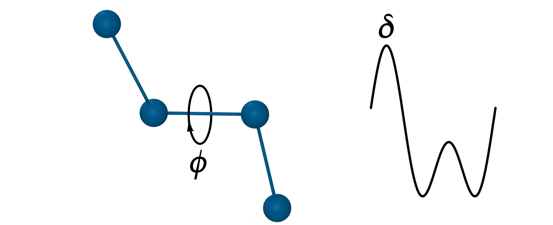
Where the non-negative integer constant n defines periodicity and \(\delta\) is the phase shift angle.
- n represents the number of potential maxima or minima generated in a 360° rotation.

Dihedrals of multiplicity of n=2 and n=3 can be combined to reproduce energy differences of cis/trans and trans/gauche conformations. The example above shows the torsion potential of ethylene glycol.
- Combination of n=2 and n=3 dihedrals used to reproduce cis/trans and trans/gauche energy differences in ethylene glycol
The improper torsion potential
Improper torsion potentials are defined for groups of 4 bonded atoms where the central atom i is connected to the 3 peripheral atoms j,k, and l. Such group can be seen as a pyramid and the improper torsion potential is related to the distance of the central atom from the base of the pyramid. This potential is used mainly to keep molecular structures planar. As there is only one energy minimum the improper torsion term can be given by a harmonic function:
- Also known as ‘out-of-plane bending’
- Defined for a group of 4 bonded atoms where the central atom i is connected to the 3 peripheral atoms j,k, and l.
- Used to enforce planarity.
- Given by a harmonic function: $V_{Improper}=k_\phi(\phi-\phi_0)^2$
$V_{Improper}=k_\phi(\phi-\phi_0)^2$

Where the dihedral angle \(\phi\) is the angle between planes ijk and ijl.
- The dihedral angle \(\phi\) is the angle between planes ijk and ijl.
Coupling Terms
The Urey-Bradley potential
It is known that as a bond angle is decreased, the adjacent bonds stretch to reduce the interaction between the outer atoms of the bonded triplet. This means that there is a coupling between bond length and bond angle. This coupling can be described by the Urey-Bradley potential. The Urey-Bradley term is defined as a (non-covalent) spring between the outer i and k atoms of a bonded triplet ijk. It is approximated by a harmonic function describing oscillation about an equilibrium distance rub with force constant kub:
- Coupling between bond length and bond angle is described by the Urey-Bradley potential.
- The Urey-Bradley term is defined as a spring between the outer atoms of a bonded triplet.
- Approximated by a harmonic function: $V_{UB}=k_{ub}(r_{jk}-r_{ub})^2$
$V_{UB}=k_{ub}(r_{ik}-r_{ub})^2$
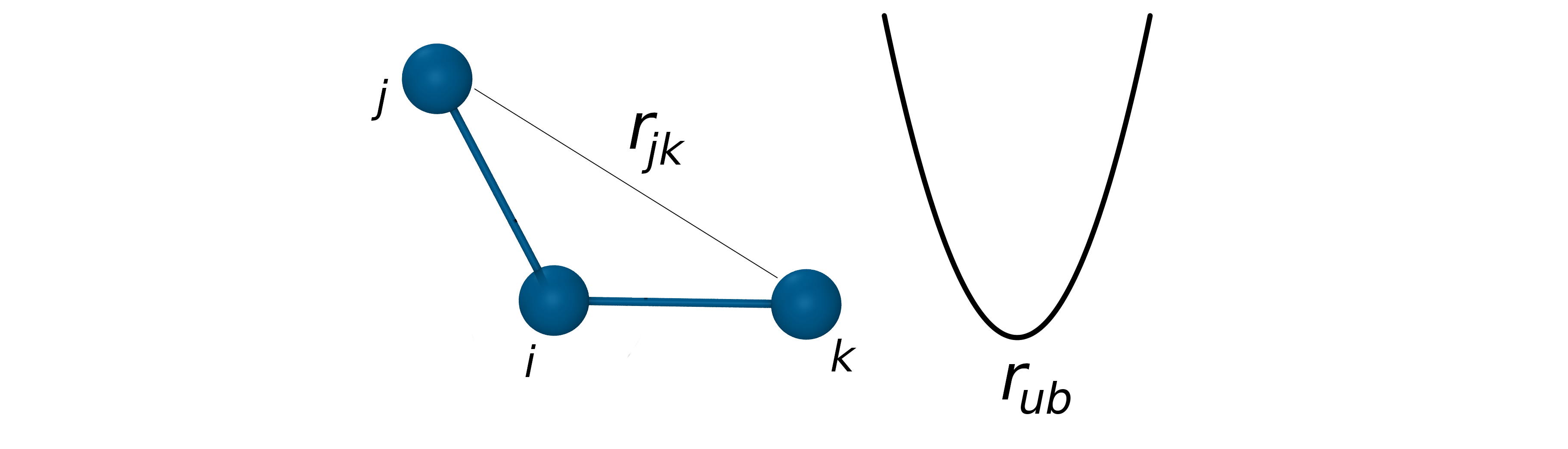
U-B terms are used to improve agreement with vibrational spectra when a harmonic bending term alone would not adequately fit. These phenomena are largely inconsequential for the overall conformational sampling in a typical biomolecular/organic simulation. The Urey-Bradley term is implemented in the CHARMM force fields.
- Improve agreement with vibrational spectra.
- Do not affect overall conformational sampling.
- Implemented in CHARMM and AMOEBA force fields.
CHARMM CMAP correction potential
A protein can be seen as a series of linked sequences of peptide units which can rotate around phi/psi angles (peptide bond N-C is rigid). These phi/psi angles define the conformation of the backbone.
- Peptide torsion angles: phi, psi, omega.
- A protein can be seen as a series of linked sequences of peptide units which can rotate around phi/psi angles.
- phi/psi angles define the conformation of the backbone.
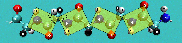
phi/psi dihedral angle potentials correct for force field deficiencies such as errors in non-bonded interactions, electrostatics, lack of coupling terms, inaccurate combination, etc.
CMAP potential is a correction map to the backbone dihedral energy. It was developed to improve the sampling of backbone conformations. CMAP parameter does not define a continuous function. it is a grid of energy correction factors defined for each pair of phi/psi angles typically tabulated with 15 degree increments.
- phi/psi dihedral angle potentials correct for force field deficiencies such as errors in non-bonded interactions, electrostatics, lack of coupling terms, inaccurate combination, etc.
- CMAP potential was developed to improve the sampling of backbone conformations.
- CMAP parameter does not define a continuous function.
- it is a grid of energy correction factors defined for each pair of phi/psi angles typically tabulated with 15 degree increments.
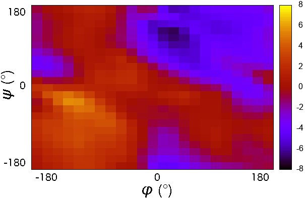
The grid of energy correction factors is constructed using QM data for every combination of \(\phi/\psi\) dihedral angles of the peptide backbone and further optimized using empirical data.
CMAP potential was initially applied to improve CHARMM22 force field. CMAP corrections were later implemented in AMBER force fields ff99IDPs (force field for intrinsically disordered proteins), ff12SB-cMAP (force field for implicit-solvent simulations), and ff19SB.
Energy scale of potential terms
| \(k_BT\) at 298 K | ~ 0.593 | \(\frac{kcal}{mol}\) |
| Bond vibrations | ~ 100 ‐ 500 | \(\frac{kcal}{mol \cdot \unicode{x212B}^2}\) |
| Bond angle bending | ~ 10 - 50 | \(\frac{kcal}{mol \cdot deg^2}\) |
| Dihedral rotations | ~ 0 - 2.5 | \(\frac{kcal}{mol \cdot deg^2}\) |
| van der Waals | ~ 0.5 | \(\frac{kcal}{mol}\) |
| Hydrogen bonds | ~ 0.5 - 1.0 | \(\frac{kcal}{mol}\) |
| Salt bridges | ~ 1.2 - 2.5 | \(\frac{kcal}{mol}\) |
Exclusions from Non-Bonded Interactions
Pairs of atoms connected by chemical bonds are normally excluded from computation of non-bonded interactions because bonded energy terms replace non-bonded interactions. In biomolecular force fields all pairs of connected atoms separated by up to 2 bonds (1-2 and 1-3 pairs) are excluded from non-bonded interactions.
Computation of the non-bonded interaction between 1-4 pairs depends on the specific force field. Some force fields exclude VDW interactions and scale down electrostatic (AMBER) while others may modify both or use electrostatic as is.
- In pairs of atoms connected by chemical bonds bonded energy terms replace non-bonded interactions.
- All pairs of connected atoms separated by up to 2 bonds (1-2 and 1-3 pairs) are excluded from non-bonded interactions. It is assumed that they are properly described with bond and angle potentials.

The 1-4 interaction turns out to be an intermediate case where both bonded and non-bonded interactions are required for a reasonable description. Due to the short distance between the 1–4 atoms full strength non-bonded interactions are too strong, and in most cases lack fine details of local internal conformational degrees of freedom. To address this problem in many cases a compromise is made to treat this particular pair partially as a bonded and partially as a non-bonded interaction.
Non-bonded interactions between 1-4 pairs depends on the specific force field. Some force fields exclude VDW interactions and scale down electrostatic (AMBER) while others may modify both or use electrostatic as is.
- 1-4 interaction represents a special case where both bonded and non-bonded interactions are required for a reasonable description. However, due to the short distance between the 1–4 atoms full strength non-bonded interactions are too strong and must be scaled down.
- Non-bonded interaction between 1-4 pairs depends on the specific force field.
- Some force fields exclude VDW interactions and scale down electrostatic (AMBER) while others may modify both or use electrostatic as is.
What Information Can MD Simulations Provide?
With the help of MD it is possible to model phenomena that cannot be studied experimentally. For example
- Understand atomistic details of conformational changes, protein unfolding, interactions between proteins and drugs
- Study thermodynamics properties (free energies, binding energies)
- Study biological processes such as (enzyme catalysis, protein complex assembly, protein or RNA folding, etc).
For more examples of the types of information MD simulations can provide read the review article: Molecular Dynamics Simulation for All.
Specifying Exclusions
GROMACS
The exclusions are generated by grompp as specified in the [moleculetype] section of the molecular topology .top file:
[ moleculetype ]
; name  nrexcl
Urea         3
...
[ exclusions ]
;  ai    aj
   1     2
   1     3
   1     4
In the example above non-bonded interactions between atoms that are no farther than 3 bonds are excluded (nrexcl=3). Extra exclusions may be added explicitly in the [exclusions] section.
The scaling factors for 1-4 pairs, fudgeLJ and fudgeQQ, are specified in the [defaults] section of the forcefield.itp file. While fudgeLJ is used only when gen-pairs is set to ‘yes’, fudgeQQ is always used.
[ defaults ]
; nbfunc        comb-rule       gen-pairs       fudgeLJ fudgeQQ
1               2               yes             0.5     0.8333
NAMD
Which pairs of bonded atoms should be excluded is specified by the exclude parameter.
Acceptable values: none, 1-2, 1-3, 1-4, or scaled1-4exclude scaled1-4 1-4scaling 0.83 scnb 2.0If scaled1-4 is set, the electrostatic interactions for 1-4 pairs are multiplied by a constant factor specified by the 1-4scaling parameter. The LJ interactions for 1-4 pairs are divided by scnb.
Key Points
Molecular dynamics simulates atomic positions in time using forces acting between atoms
The forces in molecular dynamics are approximated by simple empirical functions
Fast Methods to Evaluate Forces
Overview
Teaching: 30 min
Exercises: 0 minQuestions
Why the computation of non-bonded interactions is the speed limiting factor?
How are non-bonded interactions computed efficiently?
What is a cutoff distance?
How to choose the appropriate cutoff distance?
Objectives
Understand how non-bonded interactions are truncated.
Understand how a subset of particles for calculation of short-range non-bonded is selected.
Learn how to choose the appropriate cutoff distance and truncation method.
Learn how to select cutoff distance and truncation method in GROMACS and NAMD.
Challenges in calculation of non bonded interactions.
The most computationally demanding part of a molecular dynamics simulation is the calculation of the non-bonded terms of the potential energy function. Since the non-bonded energy terms between every pair of atoms must be evaluated, the number of calculations increases as the square of the number of atoms. In order to speed up the computation, only interactions between atoms separated by less than a preset cutoff distance are considered.
It is essential to use an efficient way of excluding pairs of atoms separated by a long distance in order to accelerate force computation. Such methods are known as “neighbour searching methods”.
- The number of non-bonded interactions increases as the square of the number of atoms.
- The most computationally demanding part of a molecular dynamics simulation is the calculation of the non-bonded interactions.
- Simulation can be significantly accelerated by limiting the number of evaluated non bonded interactions.
- Exclude pairs of atoms separated by long distance.
- Maintain a list of all particles within a predefined cutoff distance of each other.
Neighbour Searching Methods
The search for pairs of particles that are needed for calculation of the short-range non-bonded interactions is usually accelerated by maintaining a list of all particles within a predefined cutoff distance of each other.
Particle neighbours are determined either by dividing the simulation system into grid cells (cell lists) or by constructing a neighbour list for each particle (Verlet lists).
- Divide simulation system into grid cells - cell lists.
- Compile a list of neighbors for each particle by searching all pairs - Verlet lists.
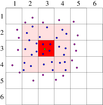
Cell Lists
The cell lists method divides the simulation domain into n cells with edge length greater or equal to the cutoff radius of the interaction to be computed. With this cell size, all particles within the cutoff will be considered. The interaction potential for each particle is then computed as the sum of the pairwise interactions between the current particle and all other particles in the same cell plus all particles in the neighbouring cells (26 cells for 3-dimensional simulation).
- Divide the simulation domain into cells with edge length greater or equal to the cutoff distance.
- Interaction potential of a particle is the sum of the pairwise interactions with all other particles in the same cell and all neighboring cells.
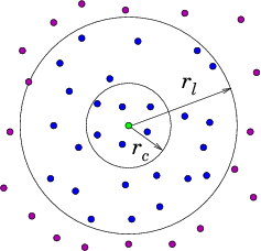
Verlet Lists
A Verlet list stores all particles within the cutoff distance of every particle plus some extra buffer distance. Although all pairwise distances must be evaluated to construct the Verlet list, it can be used for several consecutive time steps until any particle has moved more than half of the buffer distance. At this point, the list is invalidated and the new list must be constructed.
- Verlet list stores all particles within the cutoff distance plus some extra buffer distance.
- All pairwise distances must be evaluated.
- List is valid until any particle has moved more than half of the buffer distance.
Verlet offers more efficient computation of pairwise interactions at the expense of relatively large memory requirement which can be a limiting factor.
In practice, almost all simulations are run in parallel and use a combination of spatial decomposition and Verlet lists.
- Efficient computation of pairwise interactions.
- Relatively large memory requirement.
- In practice, almost all simulations use a combination of spatial decomposition and Verlet lists.
Problems with Truncation of Lennard-Jones Interactions and How to Avoid Them?
We have learned that the LJ potential is always truncated at the cutoff distance. A cutoff introduces a discontinuity in the potential energy at the cutoff value. As forces are computed by differentiating potential, a sharp difference in potential may result in nearly infinite forces at the cutoff distance (Figure 1A). There are several approaches to minimize the impact of the cutoff.
- LJ potential is always truncated at the cutoff distance.
- Truncation introduces a discontinuity in the potential energy.
- A sharp change in potential may result in nearly infinite forces.
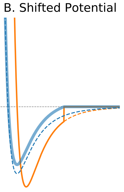
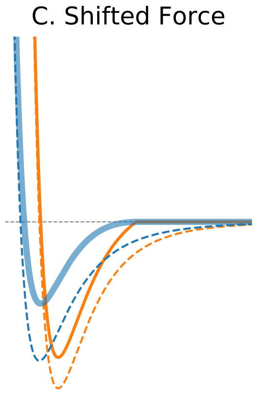
 Figure 1. The Distance Dependence of Potential and Force for Different Truncation Methods
| Shifted potential | |
The standard solution is to shift the whole potential uniformly by adding a constant at values below cutoff (shifted potential method, Figure 1B). This ensures continuity of the potential at the cutoff distance and avoids infinite forces. The addition of a constant term does not change forces at the distances below cutoff because it disappears when the potential is differentiated. However, it introduces a discontinuity in the force at the cutoff distance. Particles will experience sudden un-physical acceleration when other particles cross their respective cutoff distance. Another drawback is that when potential is shifted the total potential energy changes.</div> |
 |
| Shifted Force | |
One way to address discontinuity in forces is to shift the whole force so that it vanishes at the cutoff distance (Figure 1C). As opposed to the potential shift method the shifted forces cutoff modifies equations of motion at all distances. Nevertheless, the shifted forces method has been found to yield better results at shorter cutoff values compared to the potential shift method (Toxvaerd, 2011). |
 |
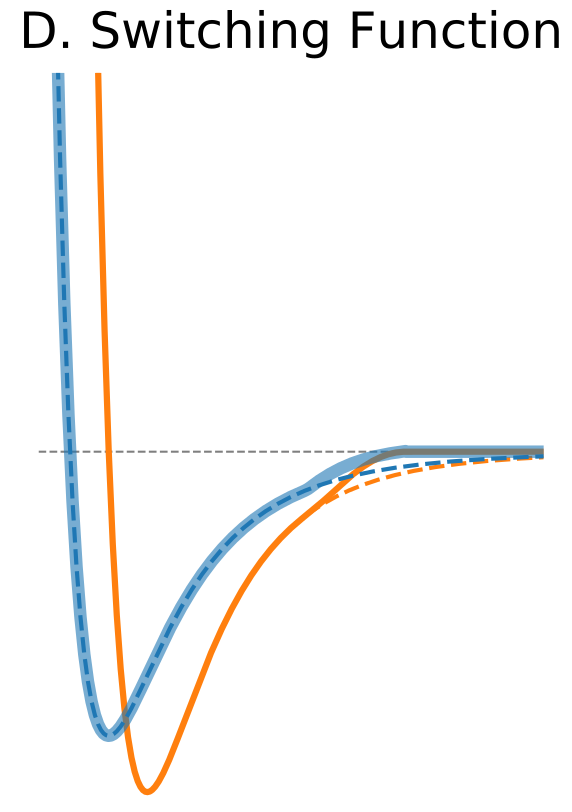
| Switching Function | |
Another solution is to modify the shape of the potential function near the cutoff boundary to truncate the non-bonded interaction smoothly at the cutoff distance. This can be achieved by the application of a switching function, for example, polynomial function of the distance. If the switching function is applied the switching parameter specifies the distance at which the switching function starts to modify the LJ potential to bring it to zero at the cutoff distance. The advantage is that the forces are modified only near the cutoff boundary and they approach zero smoothly. |
 |
| Shifted potential | |
$\circ$ Shift the whole potential uniformly by adding a constant at values below cutoff. $\circ$ Avoids infinite forces. $\circ$ Does not change forces at the distances below cutoff. $\circ$ Introduces a discontinuity in the force at the cutoff distance. $\circ$ Modifies total potential energy. |
|
| Shifted Force | |
$\circ$ Shift the whole force so that it vanishes at the cutoff distance. $\circ$ Modifies equations of motion at all distances. $\circ$ Better results at shorter cutoff values compared to the potential shift. |
|
| Switching Function | |
$\circ$ Modify the shape of the potential function near cutoff. $\circ$ Forces are modified only near the cutoff boundary and they approach zero smoothly. |
|
How to Choose the Appropriate Cutoff Distance?
A common practice is to truncate at 2.5 \(\sigma\) and this practice has become a minimum standard for truncation. At this distance, the LJ potential is about 1/60 of the well depth \(\epsilon\), and it is assumed that errors arising from this truncation are small enough. The dependence of the cutoff on \(\sigma\) means that the choice of the cutoff distance depends on the force field and atom types used in the simulation.
- A common practice is to truncate at 2.5 \(\sigma\).
- At this distance, the LJ potential is about 1/60 of the well depth \(\epsilon\).
- The choice of the cutoff distance depends on the force field and atom types.
For example for the O, N, C, S, and P atoms in the AMBER99 force field the values of \(\sigma\) are in the range 1.7-2.1, while for the Cs ions \(\sigma=3.4\). Thus the minimum acceptable cutoff, in this case, is 8.5.
In practice, increasing cutoff does not necessarily improve accuracy. There are documented cases showing opposite tendency (Yonetani, 2006). Each force field has been developed using a certain cutoff value, and effects of the truncation were compensated by adjustment of some other parameters. If you use cutoff 14 for the force field developed with the cutoff 9, then you cannot claim that you used this original forcefield. To ensure consistency and reproducibility of simulations, you should choose a cutoff that is appropriate for the force field.
- Increasing cutoff does not necessarily improve accuracy.
- Each force field has been developed using a certain cutoff value, and effects of the truncation were compensated by adjustment of some other parameters.
- To ensure consistency and reproducibility of simulation you should choose the cutoff appropriate for the force field:
Table 1. Cutoffs Used in Development of the Common Force Fields
| AMBER | CHARMM | GROMOS | OPLS |
|---|---|---|---|
| 8 Å, 10 Å (ff19SB) | 12 Å | 14 Å | 11-15 Å (depending on a molecule size) |
Properties that are very sensitive to the choice of cutoff
Different molecular properties are affected differently by various cutoff approximations. Examples of properties that are very sensitive to the choice of cutoff include the surface tension (Ahmed, 2010), the solid–liquid coexistence line (Grosfils, 2009), the lipid bi-layer properties (Huang, 2014), and the structural properties of proteins (Piana, 2012).
- the surface tension (Ahmed, 2010),
- the solid–liquid coexistence line (Grosfils, 2009),
- the lipid bi-layer properties (Huang, 2014),
- the structural properties of proteins (Piana, 2012).
For such quantities even a cutoff at 2.5 \(\sigma\) gives inaccurate results, and in some cases the cutoff must be larger than 6 \(\sigma\) was required for reliable simulations (Grosfils, 2009).
Effect of cutoff on energy conservation
Cutoff problems are especially pronounced when energy conservation is required. The net effect could be an increase in the temperature of the system over time. The best practice is to carry out trial simulations of the system under study without temperature control to test it for energy leaks or sources before a production run.
- Short cutoff may lead to an increase in the temperature of the system over time.
- The best practice is to carry out trial simulations without temperature control to test it for energy leaks or sources before a production run.
Truncation of the Electrostatic Interactions
Electrostatic interactions occurring over long distances are known to be important for biological molecules. Electrostatic interactions decay slowly and simple increase of the cutoff distance to account for long-range interactions can dramatically raise the computational cost. In periodic simulation systems, the most commonly used method for calculation of long-range electrostatic interactions is particle-mesh Ewald. In this method, the electrostatic interaction is divided into two parts: a short-range contribution, and a long-range contribution. The short-range contribution is calculated by exact summation of all pairwise interactions of atoms separated by a distance that is less than cutoff in real space. The forces beyond the cutoff radius are approximated on the grid in Fourier space commonly by the Particle-Mesh Ewald (PME) method.
- The electrostatic interaction is divided into two parts: a short-range and a long-range.
- The short-range contribution is calculated by exact summation.
- The forces beyond the cutoff radius are approximated using Particle-Mesh Ewald (PME) method.
Selecting Neighbour Searching Methods
GROMACS
Neighbour searching is specified in the run parameter file mdp.
cutoff-scheme  =  group
; Generate a pair list for groups of atoms. Since version 5.1 group list has been deprecated and only Verlet scheme is available.

cutoff-scheme  =  Verlet
; Generate a pair list with buffering. The buffer size is automatically set based on verlet-buffer-tolerance, unless this is set to -1, in which case rlist will is used.

; Neighbour search method.
ns-type = grid
; Make a grid in the box and only check atoms in neighboring grid cells.

ns-type = simple
; Loop over every atom in the box.

nstlist = 5
; Frequency to update the neighbour list. If set to 0 the neighbour list is constructed only once and never updated. The default value is 10.
NAMD
When run in parallel NAMD uses a combination of spatial decomposition into grid cells (patches) and Verlet lists with extended cutoff distance.
stepspercycle 10
# Number of timesteps in each cycle. Each cycle represents the number of timesteps between atom reassignments. Default value is 20.

pairlistsPerCycle 2
# How many times per cycle to regenerate pairlists. Default value is 2.
Selecting LJ Potential Truncation Method
GROMACS
Truncation of LJ potential is specified in the run parameter file mdp.
vdw-modifier = potential-shift
;  Shifts the VDW potential by a constant such that it is zero at the rvdw.

vdw-modifier = force-switch
;  Smoothly switches the forces to zero between rvdw-switch and rvdw.

vdw-modifier = potential-switch
;  Smoothly switches the potential to zero between rvdw-switch and rvdw.

vdw-modifier = none

rvdw-switch = 1.0
;  Where to start switching.

rvdw = 1.2
;  Cut-off distance
NAMD
Truncation of LJ potential is specified in the run parameter file mdin.
cutoff 12.0
# Cut-off distance common to both electrostatic and van der Waals calculations

switching on
# Turn switching on/off. The default value is off.

switchdist 10.0
# Where to start switching

vdwForceSwitching on
# Use force switching for VDW. The default value is off.
AMBER force fields
AMBER force fields are developed with hard truncation. Do not use switching or shifting with these force fields.
Selecting Cutoff Distance
GROMACS
Cutoff and neighbour searching is specified in the run parameter file mdp.
rlist = 1.0
; Cutoff distance for the short-range neighbour list. Active when verlet-buffer-tolerance = -1, otherwise ignored.

verlet-buffer-tolerance = 0.002
; The maximum allowed error for pair interactions per particle caused by the Verlet buffer. To achieve the predefined tolerance the cutoff distance rlist is adjusted indirectly. To override this feature set the value to -1. The default value is 0.005 kJ/(mol ps).
NAMD
When run in parallel NAMD uses a combination of spatial decomposition into grid cells (patches) and Verlet lists with extended cutoff distance.
pairlistdist 14.0
# Distance between pairs for inclusion in pair lists. Should be bigger or equal than the cutoff. The default value is cutoff.

cutoff 12.0
# Local interaction distance. Same for both electrostatic and VDW interactions.
Key Points
The calculation of non-bonded forces is the most computationally demanding part of a molecular dynamics simulation.
Non-bonded interactions are truncated to speed up simulations.
The cutoff distance should be appropriate for the force field and the size of the periodic box.
Advancing Simulation in Time
Overview
Teaching: 20 min
Exercises: 0 minQuestions
How is simulation time advanced in a molecular dynamics simulation?
What factors are limiting a simulation time step?
How to accelerate a simulation?
Objectives
Understand how simulation is advanced in time.
Learn how to choose time parameters and constraints for an efficient and accurate simulation.
Learn how to specify time parameters and constraints in GROMACS and NAMD.
Introduction
To simulate evolution of the system in time we need to solve Newtonian equations of motions. As the exact analytical solution for systems with thousands or millions of atoms is not feasible, the problem is solved numerically. The approach used to find a numerical approximation to the exact solution is called integration.
To simulate evolution of the system in time the integration algorithm advances positions of all atoms by a small step \(\delta{t}\) during which the forces are considered constant. If the time step is small enough the trajectory will be reasonably accurate. A good integration algorithm must be energy conserving. Energy conservation is important for calculation of correct thermodynamic properties. It energy is not conserved simulation may even become unstable in severe cases due to energy going to infinity. Time reversibility is important because it guarantees conservation of energy, angular momentum and any other conserved quantity. Thus good integrator for MD should be time-reversible and energy conserving.
Integration Algorithms
- To simulate evolution of the system in time we need to solve Newtonian equations of motions.
- The exact analytical solution is not feasible, the problem is solved numerically.
- The approach used to find a numerical approximation to the exact solution is called integration.
- The integration algorithm advances positions of all atoms by small time steps \(\delta{t}\).
- If the time step is small enough the trajectory will be reasonably accurate.
- A good integration algorithm for MD should be time-reversible and energy conserving.
The Euler Algorithm
The Euler algorithm is the simplest integration method. It assumes that acceleration does not change during time step. In reality acceleration is a function of coordinates, it changes when atoms move.
- The simplest integration method
The Euler algorithm uses the second order Taylor expansion to estimate position and velocity at the next time step.
Essentially this means: using the current positions and forces calculate the velocities and positions at the next time step.
- Use $\boldsymbol{r}, \boldsymbol{v},\boldsymbol{a}$ at time $t$ to compute $\boldsymbol{r}(t+\delta{t})$ and $\boldsymbol{v}(t+\delta{t})$:
$\qquad\boldsymbol{r}(t+\delta{t})=\boldsymbol{r}(t)+\boldsymbol{v}(t)\delta{t}+\frac{1}{2}\boldsymbol{a}(t)\delta{t}^2$
$\qquad\boldsymbol{v}(t+\delta{t})=\boldsymbol{v}(t)+\frac{1}{2}\boldsymbol{a}(t)\delta{t}$
Euler’s algorithm is neither time-reversible nor energy-conserving, and as such is rather unfavorable. Nevertheless, the Euler scheme can be used to integrate some other than classical MD equations of motion.
For example, GROMACS offers a Euler integrator for Brownian or position Langevin dynamics.
- Assumes that acceleration does not change during time step.
- In reality acceleration is a function of coordinates, it changes when atoms move.
Drawbacks:
- Not energy conserving
- Not reversible in time
Applications
- Not recommended for classical MD
- Can be used to integrate some other equations of motion. For example, GROMACS offers a Euler integrator for Brownian (position Langevin) dynamics.
The original Verlet Algorithm
Verlet improved the Euler integration by using positions at two successive time steps. Using positions from two time steps ensured that acceleration changes were taken into account. Essentially, this algorithm is as follows: calculate the next positions using the current positions, forces, and previous positions:
$\qquad\boldsymbol{r}(t+\delta{t})=2\boldsymbol{r}(t)-\boldsymbol{r}(t-\delta{t})+\boldsymbol{a}(t)\delta{t}^2$
- The Verlet algorithm (Verlet, 1967) requires positions at two time steps. It is inconvenient when starting a simulation when only current positions are available.
While velocities are not needed to compute trajectories, they are useful for calculating observables e.g. the kinetic energy. The velocities can only be computed once the next positions are calculated:
$\qquad\boldsymbol{v}(t+\delta{t})=\frac{r{(t+\delta{t})-r(t-\delta{t})}}{2\delta{t}}$
The Verlet algorithm is time-reversible and energy conserving.
The Velocity Verlet Algorithm
Euler integrator can be improved by introducing evaluation of the acceleration at the next time step. You may recall that acceleration is a function of atomic coordinates and is determined completely by interaction potential.
At each time step, the following algorithm is used to calculate velocity, position, and forces:
- The velocities, positions and forces are calculated at the same time using the following algorithm:
- Use $\boldsymbol{r}, \boldsymbol{v},\boldsymbol{a}$ at time $t$ to compute $\boldsymbol{r}(t+\delta{t})$: $\qquad\boldsymbol{r}(t+\delta{t})=\boldsymbol{r}(t)+\boldsymbol{v}(t)\delta{t}+\frac{1}{2}\boldsymbol{a}(t)\delta{t}^2$
- Derive $ \boldsymbol{a}(t+\delta{t})$ from the interaction potential using new positions $\boldsymbol{r}(t+\delta{t})$
- Use both $\boldsymbol{a}(t)$ and $\boldsymbol{a}(t+\delta{t})$ to compute $\boldsymbol{v}(t+\delta{t})$: $\quad\boldsymbol{v}(t+\delta{t})=\boldsymbol{v}(t)+\frac{1}{2}(\boldsymbol{a}(t)+\boldsymbol{a}(t+\delta{t}))\delta{t} $
- The Verlet algorithm is time-reversible and energy conserving.
Mathematically, Velocity Verlet is equivalent to the original Verlet algorithm. Unlike the basic Verlet algorithm, this algorithm explicitly incorporates velocity, eliminating the issue of the first time step.
The Velocity Verlet algorithm is mathematically equivalent to the original Verlet algorithm. It explicitly incorporates velocity, solving the problem of the first time step in the basic Verlet algorithm.
- The Velocity Verlet algorithm is the most widely used algorithm in MD simulations because of its simplicity and stability
- Due to its simplicity and stability the Velocity Verlet has become the most widely used algorithm in the MD simulations.
Leap Frog Variant of Velocity Verlet
The Leap Frog algorithm is essentially the same as the Velocity Verlet. The Leap Frog and the Velocity Verlet integrators give equivalent trajectories. The only difference is that the velocities are not calculated at the same time as positions. Leapfrog integration is equivalent to updating positions and velocities at interleaved time points, staggered in such a way that they “leapfrog” over each other. The only practical difference between the velocity Verlet and the leap-frog is that restart files are different.
- The leap frog algorithm is a modified version of the Verlet algorithm.
- The only difference is that the velocities are not calculated at the same time as positions.
- Positions and velocities are computed at interleaved time points, staggered in such a way that they “leapfrog” over each other.
Velocity, position, and forces are calculated using the following algorithm:
- Derive $ \boldsymbol{a}(t)$ from the interaction potential using positions $\boldsymbol{r}(t)$
- Use $\boldsymbol{v}(t-\frac{\delta{t}}{2})$ and $\boldsymbol{a}(t)$ to compute $\boldsymbol{v}(t+\frac{\delta{t}}{2})$: $\qquad\boldsymbol{v}(t+\frac{\delta{t}}{2})=\boldsymbol{v}(t-\frac{\delta{t}}{2}) + \boldsymbol{a}(t)\delta{t}$
- Use current $\boldsymbol{r}(t)$ and $\boldsymbol{v}(t+\frac{\delta{t}}{2})$ to compute $\boldsymbol{r}(t+\delta{t})$ : $\qquad\boldsymbol{r}(t+\delta{t})=\boldsymbol{r}(t)+\boldsymbol{v}(t+\frac{\delta{t}}{2})\delta{t}$
- The Leap Frog and the Velocity Verlet integrators give equivalent trajectories.
- Restart files are different
Discontinuities in simulations occur when the integrator is changed
Since velocities in Leap-frog restart files are shifted by half a time step from coordinates, changing the integrator to Verlet will introduce some discontinuity.
Integrator pairs of coordinates ($r$) and velocities ($v$) Velocity-Verlet $[r_{t=0}, v_{t=0}], [r_{t=1}, v_{t=1}], [r_{t=2}, v_{t=2}], \ldots $ Leap-Frog $[r_{t=0}, v_{t=0.5}], [r_{t=1}, v_{t=1.5}], [r_{t=2}, v_{t=2.5}], \ldots $ A simulation system will experience an instantaneous change in kinetic energy. That makes it impossible to transition seamlessly between integrators.
Selecting the Integrator
GROMACS
Several integration algorithms available in GROMACS are specified in the run parameter mdp file.
integrator = md
; A leap frog algorithm

integrator = md-vv
;  A velocity Verlet algorithm

integrator = md-vv-avek
; A velocity Verlet algorithm same as md-vv except the kinetic energy is calculated as the average of the two half step kinetic energies. More accurate than the md-vv.

integrator = sd
;  An accurate leap frog stochastic dynamics integrator.

integrator = bd
; A Euler integrator for Brownian or position Langevin dynamics.
NAMD
The only available integration method is Verlet.
How to Choose Simulation Time Step?
Larger time step allows to run simulation faster, but accuracy decreases.
Mathematically Verlet family integrators are stable for time steps:
\(\qquad\delta{t}\leq\frac{1}{\pi{f}}\qquad\) where \(f\) is oscillation frequency.
- Verlet family integrators are stable for time steps: \(\delta{t}\leq\frac{1}{\pi{f}}\) where \(f\) is oscillation frequency.
In molecular dynamics stretching of the bonds with the lightest atom H is usually the fastest motion. The period of oscillation of a C-H bond is about 10 fs. Hence Verlet integration will be stable for time steps < 3.2 fs. In practice, the time step of 1 fs is recommended to describe this motion reliably.
- Vibrations of bonds with hydrogens have period of 10 fs
- Bond vibrations involving heavy atoms and angles involving hydrogen atoms have period of 20 fs
If the dynamics of hydrogen atoms is not essential for a simulation, bonds with hydrogens can be constrained. By replacing bond vibrations with holonomic (not changing in time) constraints the simulation step can be doubled since the next fastest motions (bond vibrations involving only heavy atoms and angles involving hydrogen atoms) have a period of about 20 fs. Further increase of the simulation step requires constraining bonds between all atoms and angles involving hydrogen atoms. Then the next fastest bond vibration will have 45 fs period allowing for another doubling of the simulation step.
To accelerate a simulation the electrostatic interactions outside of a specified cutoff distance can be computed less often than the short range bonded and non-bonded interactions. It is also possible to employ an intermediate timestep for the short-range non-bonded interactions, performing only bonded interactions every timestep.
- Stretching of bonds with the lightest atom H is the fastest motion.
- As period of oscillation of a C-H bond is about 10 fs, Verlet integration is stable for time steps < 3.2 fs.
- In practice, the time step of 1 fs is recommended to describe this motion reliably.
- Simulation step can be doubled by constraining bonds with hydrogens.
- Further increase of the simulation step requires constraining bonds between all atoms and angles involving hydrogen atoms.
Other ways to increase simulation speed
- Compute long range electrostatic interactions less often than the short range interactions.
- Employ an intermediate timestep for the short-range non-bonded interactions, performing only bonded interactions at each timestep.
- Hydrogen mass repartitioning allows increasing time step to 4 fs.
Specifying Time Parameters
GROMACS
Time parameters are specified in the mdp run parameter file.
dt = 0.001
; Time step, ps

nsteps = 10000
; Number of steps to simulate

tinit = 0
; Time of the first step
NAMD
Time parameters are specified in the mdin run parameter file.
TimeStep = 1
# Time step, fs

NumSteps = 10000
# Number of steps to simulate

FirstTimeStep = 0
# Time of the first step

#  Multiple time stepping parameters
nonbondedFreq 2
#  Number of timesteps between short-range non-bonded evaluation.

fullElectFrequency 4
# Number of timesteps between full electrostatic evaluations
Constraint Algorithms
To constrain bond length in a simulation the equations of motion must be modified. Constraint forces acting in opposite directions along a bond are usually applied to accomplish this. The total energy of the simulation system is not affected in this case because the total work done by constraint forces is zero. In constrained simulation, the unconstrained step is performed first, then corrections are applied to satisfy constraints.
- To constrain bond length in a simulation the equations of motion must be modified.
- The goal is to constrain some bonds without affecting dynamics and energetics of a system.
- One way to constrain bonds is to apply constraint force acting along a bond in opposite direction.
In constrained simulation first the unconstrained step is done, then corrections are applied to satisfy constraints.
Since bonds in molecules are coupled, satisfying all constraints is a complex nonlinear problem. Is it fairly easy to solve it for a small molecule like water but as the number of coupled bonds increases, the problem becomes more difficult. Several algorithms have been developed for use specifically with small or large molecules.
- As bonds in molecules are coupled satisfying all constraints in a molecule becomes increasingly complex for larger molecules.
- Several algorithms have been developed for use specifically with small or large molecules.
SETTLE
SETTLE is very fast analytical solution for small molecules. It is widely used to constrain bonds in water molecules.
- Very fast analytical solution for small molecules.
- Widely used to constrain bonds in water molecules.
SHAKE
SHAKE is an iterative algorithm that resets all bonds to the constrained values sequentially until the desired tolerance is achieved. SHAKE is simple and stable, it can be applied for large molecules and it works with both bond and angle constraints. However it is substantially slower than SETTLE and hard to parallelize. SHAKE may fail to find the constrained positions when displacements are large. The original SHAKE algorithm was developed for use with a leap-frog integrator. Later on, the extension of SHAKE for use with a velocity Verlet integrator called RATTLE has been developed. Several other extensions of the original SHAKE algorithm exist (QSHAKE, WIGGLE, MSHAKE, P-SHAKE).
- Iterative algorithm that resets all bonds to the constrained values sequentially until the desired tolerance is achieved.
- Simple and stable, it can be applied for large molecules.
- Works with both bond and angle constraints.
- Slower than SETTLE and hard to parallelize.
- SHAKE may fail to find the constrained positions when displacements are large.
Extensions of the original SHAKE algorithm: RATTLE, QSHAKE, WIGGLE, MSHAKE, P-SHAKE.
LINCS
LINCS algorithm (linear constraint solver), employs a power series expansion to determine how to move the atoms such that all constraints are satisfied. It is 3-4 times faster than SHAKE and easy to parallelize. The parallel LINCS (P-LINCS) allows to constrain all bonds in large molecules. The drawback is that it is not suitable for constraining both bonds and angles.
- Linear constraint solver
- 3-4 times faster than SHAKE and easy to parallelize.
- The parallel LINCS (P-LINCS) allows to constrain all bonds in large molecules.
- Not suitable for constraining both bonds and angles.
Specifying Constraints
GROMACS
SHAKE, LINCS and SETTLE constraint algorithms are implemented. They are selected via keywords in mdp input files
constraints = h-bonds
; Constrain bonds with hydrogen atoms

constraints = all-bonds
; Constrain all bonds

constraints = h-angles
; Constrain all bonds and additionally the angles that involve hydrogen atoms

constraints = all-angles
; Constrain all bonds and angles

constraint-algorithm = LINCS
; Use LINCS

constraint-algorithm = SHAKE
; Use SHAKE

shake-tol = 0.0001
;  Relative tolerance for SHAKE, default value is 0.0001.
SETTLE can be selected in the topology file:
[ settles ]
; OW    funct   doh     dhh
1       1       0.1     0.16333
NAMD
SHAKE and SETTLE constraint algorithms are implemented. They are selected via keywords in simulation input file.
rigidBonds water
# Use SHAKE to constrain bonds with hydrogens in water molecules.

rigidBonds all
# Use SHAKE to constrain bonds with hydrogens in all molecules.

rigidBonds none
# Do not constrain bonds. This is the default.

rigidTolerance 1.0e-8
# Stop iterations when all constrained bonds differ from the nominal bond length by less than this amount. Default value is 1.0e-8.

rigidIterations 100
# The maximum number of iterations. If the bond lengths do not converge, a warning message is emitted. Default value is 100.

rigidDieOnError on
# Exit and report an error if rigidTolerance is not achieved after rigidIterations. The default value is on.

useSettle on
# If rigidBonds are enabled then use the SETTLE algorithm to constrain waters. The default value is on.
Key Points
A good integration algorithm for MD should be time-reversible and energy conserving.
The most widely used integration method is the velocity Verlet.
Simulation time step must be short enough to describe the fastest motion.
Time step can be increased if bonds involving hydrogens are constrained.
Additional time step increase can be achieved by constraining all bonds and angles involving hydrogens.
Periodic Boundary Conditions
Overview
Teaching: 20 min
Exercises: 0 minQuestions
How to simulate a bulk (gas, liquid or solid) system by using only a small part?
Objectives
Understand why and when periodic boundary conditions are used.
Understand how shape and size of a periodic box can affect simulation.
Learn how to set periodic box parameters in GROMACS and NAMD.
What is PBC and why is it important?
In most cases we want to simulate a system in realistic environment, such as solution. If one tries to simulate a protein in a droplet of water, it will simply evaporate.
The boundary to contain molecules in simulation is needed to preserve thermodynamic properties like temperature, pressure and density. The use of PBC in simulations allows the inclusion of bulk solvent or crystalline environments. In other words periodic boundary conditions make it possible to approximate an infinite system by using a small part (unit cell). A unit cell in MD is usually referred to as periodic box.
- In most cases we want to simulate a system in realistic environment, such as solution.
- Try simulating a droplet of water, it will simply evaporate.
- We need a boundary to contain water and control temperature, pressure, and density.
- Periodic boundary conditions allow to approximate an infinite system by using a small part (unit cell).

To implement PBC the unit cell is surrounded by translated copies in all directions to approximate an infinitely large system. When one molecule diffuses across the boundary of the simulation box it reappears on the opposite side. So each molecule always interacts with its neighbours even though they may be on opposite sides of the simulation box. This approach replaces the surface artifacts caused by the interaction of the isolated system with a vacuum with the PBC artifacts which are in general much less severe.
- Unit cell is surrounded by an infinite number of translated copies in all directions (images).
- When a particle in unit cell moves across the boundary it reappears on the opposite side.
- Each molecule always interacts with its neighbors even though they may be on opposite sides of the simulation box.
- Artifacts caused by the interaction of the isolated system with a vacuum are replaced with the PBC artifacts which are in general much less severe.
Choosing periodic box size and shape.
Box shape
Cubic periodic box
A cubic box is the most intuitive and common choice, but it is inefficient due to irrelevant water molecules in the corners. The extra water will make your simulation run slower.
- A cubic box is the most intuitive and common choice
- Cubic box is inefficient due to irrelevant water molecules in the corners.

Ideally you need a sufficiently large sphere of water surrounding the macromolecule, but that’s impossible because spheres can’t be packed to fill space.
- Ideal simulation system is a sphere of water surrounding the macromolecule, but spheres can’t be packed to fill space.
Octahedral and dodecahedral periodic boxes
A common alternatives that are closer to spherical are the dodecahedron (any polyhedron with 12 faces) or the truncated octahedron (14 faces). These shapes work reasonably well for globular macromolecules.
- The dodecahedron (12 faces) or the truncated octahedron (14 faces) are closer to sphere.
| Space filling with truncated octahedrons | |
|---|---|
 |
 |
- These shapes work reasonably well for globular macromolecules.
Triclinic periodic boxes
The triclinic box is the least symmetric of all types of periodic boxes. The triclinic system defines the unit cells by three basis vectors of unequal length, and the angles between these vectors must all be different from each other, and not 90 degrees.
In simulation packages, however, there usually are no such restrictions for triclinic boxes, which is why they are the most generic periodic boundary conditions. Any periodic box can be converted into a triclinic box with specific box vectors and angles.
- Any repeating shape that fills all of space has an equivalent triclinic unit cell.
- A periodic box of any shape can be represented by a triclinic box with specific box vectors and angles.
There are two reasons why triclinic boxes are useful: First, they can be used to simulate crystals that don’t have rectangular unit cells. In addition, the best triclinic cell has about 71% the volume of an ideal rectangular cell.
- The optimal triclinic cell has about 71% the volume of the optimal rectangular cell.
Box size
A good rule of thumb is to keep the box at least 10 Å away from the solute. Of course this assumes completely equilibrated system. If you are preparing a new system, make sure there is at least a margin of 13 Å between the solvent and the box, since the solvent will come closer to the solute during equilibration and the box will contract.
- The minimum box size should extend at least 10 nm from the solute.

In order to avoid short range interactions between a molecule and its images, the shortest periodic box vector should be at least twice as big as the cuf-off radius.
- The shortest periodic box vector should be at least twice bigger than the cuf-off radius.

The solvent molecules in simulations involving macromolecules should not “feel” both sides of a solute. In other words, there must be at least twice the cut-off distance between a macromolecule and any of its images.
- In simulations with macromolecules solvent molecules should not “feel” both sides of a solute.
When your simulation system is small make sure you do not set the cutoff too high!

Pitfalls
Solvated macromolecules rotate during simulations. Furthermore macromolecules may undergo conformational changes. Often these changes are of major interest and should not be restricted in any way.
Periodic boxes for elongated molecules are also elongated when the distance between the solute and the box is used to prepare them. If the smallest box dimension is not large enough rotation will result in the interaction between the molecule and its periodic images and lead to unphysically restricted dynamics. Thus, when setting up a periodic system, you must consider rotation of elongated macromolecules as well as possible changes in conformation.
Use of a cubical or dodecahedral box is one way to solve this problem. A disadvantage of such an approach is that you will need a lot of water to fill the box.
- A simulation system with elongated solute in cubic or dodecahedral box will have a large amount of water located far away from the solute.
- Consider using a narrow rectangular box.
- Rotation of elongated macromolecules and/or conformational changes must be taken in consideration.

Using a narrow box together with constraining rotational motion is more efficient [1]. Be aware, however, that the box shape itself may impact conformational dynamics by restricting motion in certain directions [2]. This effect may be significant when the amount of solvent is minimal.
- Constrain the rotational motion.
- The box shape itself may influence conformational dynamics by restricting motions in certain directions.
Specifying Periodic Box
GROMACS
The box specification is integrated into structure files. The box parameters can be set using the editconf program or manually. The editconf program accepts the following options:
-bt Box type triclinic, cubic, dodecahedron, octahedron -box Box vectors lengths, a, b, c nm -angles Box vectors angles, bc, ac, ab degrees -d Distance between the solute and the box nm Example:
module load StdEnv/2020 gcc gromacs
wget http://files.rcsb.org/view/1lyz.pdb
gmx pdb2gmx -f 1lyz.pdb -ff amber99sb-ildn -water spce -ignh
gmx editconf -f conf.gro -o conf_boxed.gro -d 1.0 -bt cubic
In the example above the editconf program will append box vectors to the structure file ‘conf.gro’ and save it in the file ‘conf_boxed.gro’. The 9 components of the three box vectors are saved in the last line of the structure file in the order: xx yy zz xy xz yx yz zx zy. Three of the values (xy, xz, and yz) are always zeros because they are duplicates of (yx, zx, and zy). The values of the box vectors components are related to the unit cell vectors \(a,b,c,\alpha,\beta,\gamma\) from the CRYST1 record of a PDB file with the equations:
\[xx=a, yy=b\cdot\sin(\gamma), zz=\frac{v}{(a*b*\sin(\gamma))}\] \[xy=0, xz=0, yx=b\cdot\cos(\gamma)\] \[yz=0, zx=c\cdot\cos(\beta), zy=\frac{c}{\sin(\gamma)}\cdot(cos(\alpha)-cos(\beta)\cdot\cos(\gamma))\] \[v=\sqrt{1-\cos^2(\alpha)-cos^2(\beta)-\cos^2(\gamma) +2.0\cdot\cos(\alpha)\cdot\cos(\beta)\cdot\cos(\gamma)}\cdot{a}\cdot{b}\cdot{c}\]NAMD
Periodic box is specified in the run parameter file by three unit cell vectors, the units are Å.
# cubic box
cellBasisVector1 100 0 0
cellBasisVector2 0 100 0
cellBasisVector3 0 0 100
Alternatively periodic box parameters can be read from the .xsc (eXtended System Configuration) file by using the extendedSystem keyword. If this keyword is used cellBasisVectors are ignored. NAMD always generates .xsc files at runtime.
extendedSystem restart.xsc
Comparing periodic boxes
Using the structure file ‘conf.gro’ from the example above generate triclinic, cubic, dodecahedral and truncated octahedral boxes with the 15 Å distance between the solute and the box edge.
Which of the boxes will be the fastest to simulate?
References:
- Molecular dynamics simulations with constrained roto-translational motions: Theoretical basis and statistical mechanical consistency
- The effect of box shape on the dynamic properties of proteins simulated under periodic boundary conditions
- Periodic box types in Gromacs manual
Key Points
Periodic boundary conditions are used to approximate an infinitely large system.
Periodic box should not restrict molecular motions in any way.
The macromolecule shape, rotation and conformational changes should be taken into account in choosing the periodic box parameters.
Degrees of Freedom
Overview
Teaching: 10 min
Exercises: 0 minQuestions
How is kinetic energy contained and distributed in a dynamic molecular system
Why constraints are used in MD simulations, and how they can affect dynamics
Objectives
Molecular degrees of freedom
Molecular degrees of freedom refer to the number of unique ways a molecule may move (increase its kinetic energy). Thus the molecular degrees of freedom describe how kinetic energy is contained and distributed in a molecule. Dynamical molecular systems are characterized by numerous degrees of freedom. The motion of molecules can be decomposed into translational, rotational, and vibrational components.
- The number of unique ways a molecule may move (increase its kinetic energy).
- Describe how kinetic energy is contained and distributed in a molecule.
- Translational, rotational, and vibrational components.
Equipartition theorem
On average, when thermal energy is added to a system, the energy is shared equally among the degrees of freedom (equipartition theorem). In other words, classical equipartition principle states that every (quadratic) degree of freedom contributes equally to the total energy in thermal equilibrium. Each degree of freedom has an average energy of \(\frac{1}{2}k_BT\) and contributes \(\frac{1}{2}k_B\) to the system’s heat capacity.
- The energy is shared equally among the degrees of freedom (equipartition theorem).
- Each degree of freedom has an average energy of \(\frac{1}{2}k_BT\) and contributes \(\frac{1}{2}k_B\) to the system’s heat capacity.
Degrees of freedom and thermodynamics properties
When the same amount of kinetic energy flows into simulation systems containing different types of molecules, their temperature will change by a different amount. The more places (degrees of freedom) there are to put the energy the less the temperature change will be.
The number of degrees of freedom is an important quantity allowing us to estimate various thermodynamic variables for a simulation system (for example heat capacity, entropy, temperature).
- When kinetic energy is applied to simulation systems containing molecules with different degrees of freedom, the temperature increase will vary.
- If energy is spread over many places (degrees of freedom), the temperature will change less.
- The number of degrees of freedom is an essential quantity for estimating various thermodynamic variables for a simulation system (such as heat capacity, entropy, and temperature).
Translational degrees of freedom
An atom or a molecule can move in three dimensions. Thus, any atom or molecule has three degrees of freedom associated with translational motion of the center of mass with respect to the X, Y, and Z axes.
- The three translational degrees of freedom in three dimensions provide \(\frac{3}{2}k_BT\) of energy.
- Atoms and molecules have three degrees of freedom associated with the translation of their centers of mass about each coordinate axis.
- Translational degrees of freedom in three dimensions yield \(\frac{3}{2}k_BT\) of energy.
Rotational degrees of freedom
From the classical point of view atoms have a negligible amount of rotational energy because their mass is concentrated in the nucleus. Since radius of a nucleus is about \(10^{-15}\) m, atoms have negligible rotational moment of inertia. (From the QM point of view rotation of an atom has no meaning because such rotations lead to configurations which are indistinguishable from the original configuration). But molecules are different in this respect, they can have rotational kinetic energy. A linear molecule, has two rotational degrees of freedom, because it can rotate about either of two axes perpendicular to the molecular axis. The rotations along the molecular axis have a negligible amount of rotational energy because the mass is concentrated very close to the axis of rotation. A nonlinear molecule, where the atoms do not lie along a single axis, like water, has three rotational degrees of freedom, because it can rotate around any of three perpendicular axes.
- The rotational degrees of freedom contribute \(k_BT\) to the energy of linear molecules and \(\frac{3}{2}k_BT\) to the energy of non-linear molecules.
- Atoms have a negligible amount of rotational energy because their mass is concentrated in the nucleus which is very small (about \(10^{-15}\) m).
- A linear molecule, has two rotational degrees of freedom.
- A nonlinear molecule, where the atoms do not lie along a single axis, has three rotational degrees of freedom, because it can rotate around any of three perpendicular axes.
- The rotational degrees of freedom contribute \(k_BT\) to the energy of linear molecules and \(\frac{3}{2}k_BT\) to the energy of non-linear molecules.
Vibrational degrees of freedom
A molecule can also vibrate. A diatomic molecule has one molecular vibration mode, where the two atoms oscillate back and forth with the chemical bond between them acting as a spring.
A molecule with N atoms has more complicated modes of molecular vibration, with 3N − 5 vibrational modes for a linear molecule and 3N − 6 modes for a nonlinear molecule.
- A diatomic molecule has one molecular vibration mode.
- A linear molecule with N atoms has 3N − 5 vibrational modes.
- A non-linear molecule with N atoms has 3N − 6 vibrational modes.
| Angle bend | Symmetric stretch | Asymmetric stretch |
|---|---|---|
 |
 |
 |
Each vibrational mode has two degrees of freedom for energy. The kinetic energy of moving atoms is one degree of freedom, and the potential energy of spring-like chemical bonds is another.
Each vibrational degree of freedom provides \(k_BT\) of energy. However, this is valid only when \(k_BT\) is much bigger than spacing between vibrational states. At low temperature this condition is not satisfied, only a few vibrational states are occupied and the equipartition principle is not typically applicable.
- There are two degrees of freedom for each vibrational mode.
- One degree involves the kinetic energy of the moving atoms, and the other involves the potential energy of the springlike chemical bond(s).
- Each vibrational degree of freedom contributes \(k_BT\) to the energy of a molecule. However, this is valid only when \(k_BT\) is much bigger than energy spacing between vibrational modes.
- At low temperature this condition is not satisfied, only a few vibrational states are occupied and the equipartition principle is not typically applicable.
Increasing efficiency of thermodynamic sampling.
To compute thermodynamic quantities with a molecular simulation, we sample a configuration space with the dimensionality determined by the number of degrees of freedom. Thus, by reducing the number of degrees of freedom (of course when physically justifiable) we can increase thermodynamic sampling efficiency.
By reducing the number of degrees of freedom we can increase thermodynamic sampling efficiency.
Constraints are used in most molecular dynamics simulations, since the maximum length of the time step for integrating the equations of motion is limited by the frequency of the fastest motions in the system. Bond constraints that remove the rapid vibrational modes eliminate those degrees of freedom and make possible to use longer time steps without losing conservation of energy. Constraints including angles and dihedrals can be also applied.
- Force fields remove the electrons’ degrees of freedom by replacing them with atom centered charges.
- An implicit solvent model eliminates the degrees of freedom associated with the solvent molecules.
- Bond constraints eliminate vibrational degrees of freedom and make possible to use longer time steps.
- Constraints including angles and dihedrals can be also applied.
Reduction of the number of degrees of freedom may lead to artifacts.
Applying constraints, however, can affect the simulation by restricting the motions associated with the specified degrees of freedom. For example it was found that bond and angle constraints slow down dihedral angle transitions (Toxvaerd, 1987), shift the frequencies of the normal modes in biomolecules (Tobias and Brooks, 1988), and perturb the dynamics of polypeptides (Hinsen and Kneller, 1995).
Bond and angle constraints can:
- slow down dihedral angle transitions [1]
- shift the frequencies of the normal modes in biomolecules [2]
- perturb the dynamics of polypeptides [3].
Key Points
Degrees of Freedom in Rigid bodies.
Constraints decrease the number of degrees of freedom
Imposing constraints can affect simulation outcome
Electrostatic Interactions
Overview
Teaching: 10 min
Exercises: 0 minQuestions
How electrostatic interactions are calculated in periodic systems?
Objectives
Learn what parameters control the accuracy of electrostatic calculations
Coulomb interactions
- Long range: $V_{Elec}=\frac{q_{i}q_{j}}{4\pi\epsilon_{0}\epsilon_{r}r_{ij}}$
Due to the long-range behavior of Coulomb interactions, the task of computing Coulomb potentials is often the most time consuming part of any MD simulation. Therefore, fast and efficient algorithms are required to accelerate these calculations.
- Computing Coulomb potentials is often the most time consuming part of any MD simulation.
- Fast and efficient algorithms are required for these calculations.
Particle Mesh Ewald (PME)
Particle Mesh Ewald (PME) method is the most widely used method using the Ewald decomposition technique. The potential is decomposed into two parts: a fast decaying and a slow decaying. A fast decaying part is computed in real space. A slow decaying part is computed in Fourier space (reciprocal space).
- The most widely used method using the Ewald decomposition.
- The potential is decomposed into two parts: fast decaying and slow decaying.

Fast decaying short-ranged potential (Particle part).
The real space sum is short-ranged and as for the LJ potentials, it can be truncated when sufficiently decayed. It is a direct sum of contributions from all particles within a cutoff radius. It is the Particle part of PME.
- Sum of all pairwise Coulomb interactions within a cutoff radius
- Implements same truncation scheme as the LJ potentials.
Slow decaying long-ranged potential (Mesh part).
The Fourier space part, on the other hand, is long-ranged but smooth and periodic. This part is a slowly varying function. PME takes advantage of the fact that all periodic functions can be represented with a sum of sine or cosine components, and slowly varying functions can be accurately described by only a limited number of low frequency components (k vectors). In other words Fourier transform of the long-range Coulomb interaction decays rapidly in Fourier space, and summation converges fast.
- Slowly varying, smooth and periodic function.
- All periodic functions can be represented with a sum of sine or cosine components.
- Slowly varying functions can be accurately described by only a limited number of low frequency components (k vectors).
PME algorithm
The long range contribution can then be efficiently computed in Fourier space using FFT. Fourier transform calculation is discrete and requires the input data to be on a regular grid. It is the Mesh part of PME. As point charges in a simulation are non-equispaced, they need to be interpolated to obtain charge values in equispaced grid cells.
- Long-range electrostatic interactions are evaluated using 3-D grids in reciprocal Fourier space.
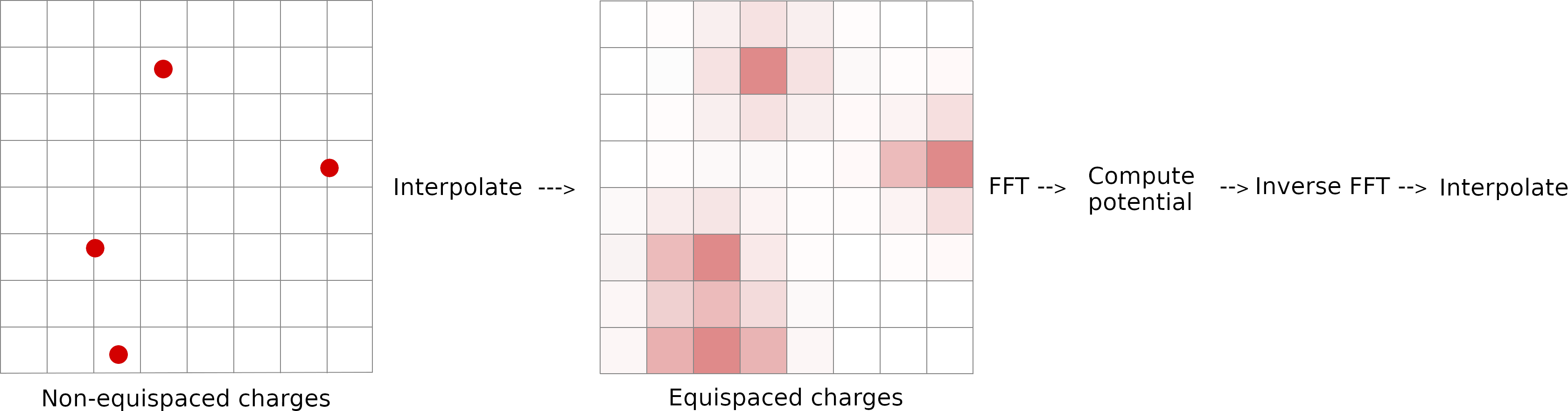
- Assign charges to grid cells. Charges in grid cells are obtained by interpolation.
- Compute Fourier transform.
- Compute potential. Coulomb interaction decays rapidly in Fourier space, and summation converges fast.
- Compute inverse Fourier transform.
- Interpolate gridded potentials back to atomic centers.
Simulation parameters controlling speed and accuracy of PME calculations.
- Grid spacing and dimension. Grid dimension values give the size of the charge grid (upon which the reciprocal sums are interpolated) in each dimension. Higher values lead to higher accuracy (when the direct space tolerance is also lowered) but considerably slow down the calculation. Generally it has been found that reasonable results are obtained when grid dimension values are approximately equal to periodic box size, leading to a grid spacing of 1.0 Å. Significant performance enhancement in the calculation of the fast Fourier transform is obtained by having each of the values be a product of powers of 2, 3, and/or 5. If the values are not given, programs will chose values to meet these criteria.
- Direct space tolerance. Controls the splitting into direct and reciprocal part. Higher tolerance shifts more charges into Fourier space.
- Interpolation order is the order of the B-spline interpolation. The higher the order, the better the accuracy (unless the charge grid is too coarse). The minimum order is 3. An order of 4 (the default) implies a cubic spline approximation which is a good standard value.
- Grid spacing. Lower values lead to higher accuracy but considerably slow down the calculation. Default 1.0 Å.
- Grid dimension. Higher values lead to higher accuracy but considerably slow down the calculation.
- Direct space tolerance. Controls the splitting into direct and reciprocal part. Higher tolerance shifts more charges into Fourier space.
- Interpolation order is the order of the B-spline interpolation. The higher the order, the better the accuracy. Default 4 (cubic spline).
| Variable \ MD package | GROMACS | NAMD | AMBER |
|---|---|---|---|
| Fourier grid spacing | fourierspacing (1.2) | PMEGridSpacing (1.5) | |
| Grid Dimension X | fourier-nx | PMEGridSizeX | nfft1 |
| Grid Dimension Y | fourier-ny | PMEGridSizeY | nfft2 |
| Grid Dimension Z | fourier-nz | PMEGridSizeZ | nfft3 |
| Direct space tolerance | ewald-rtol (\(10^{-5}\)) | PMETolerance (\(10^{-5}\)) | dsum_tol (\(10^{-6}\)) |
| Interpolation order | pme-order (4) | PMEInterpOrder (4) | order (4) |
| Variable \ MD package | GROMACS | NAMD | AMBER |
|---|---|---|---|
| Fourier grid spacing | fourierspacing (1.2) | PMEGridSpacing (1.5) | |
| Grid Dimension [X,Y,Z] | fourier-[nx,ny,nz] | PMEGridSize[X,Y,Z] | nfft[1,2,3] |
| Direct space tolerance | ewald-rtol (\(10^{-5}\)) | PMETolerance (\(10^{-5}\)) | dsum_tol (\(10^{-6}\)) |
| Interpolation order | pme-order (4) | PMEInterpOrder (4) | order (4) |
Key Points
Calculation of electrostatic potentials is the most time consuming part of any MD simulation
Long-range part of electrostatic interactions is calculated by approximating Coulomb potentials on a grid
Denser grid increases accuracy, but significantly slows down simulation
Controlling Temperature
Overview
Teaching: 20 min
Exercises: 0 minQuestions
What is temperature on the molecular level?
Why do we want to control the temperature of our MD-simulations?
What temperature control algorithms are commonly used?
What are the strengths and weaknesses of these common thermostats?
Objectives
Remind us how Maxwell-Boltzmann distributions relate to temperature.
Quickly review thermodynamic ensembles.
Learn about different thermostats and get an idea how they work.
Learn where thermostats that don’t produce correct thermodynamic ensembles can still be very useful.
Temperature at the molecular level.
Temperature is a macroscopic property and thermodynamics tells us that on the molecular level, the temperature of a system is defined by the average kinetic energy of all the particles (atoms, molecules) that make up the system. Statistical thermodynamics tells us that a system that contains a certain amount of energy and is in equilibrium, will have all of its energy distributed in the most probable way. This distribution is called the Maxwell-Boltzmann distribution. This means that in a system of particles, these particles won’t all have the same velocity but rather the velocities will follow a distribution that depends on their mass and the temperature of the system.
- Temperature is defined by the average kinetic energy of all the particles.
- A system in equilibrium, will have all of its energy distributed in the most probable way.
- Particles in a system at equilibrium don’t all have the same velocity.
- Velocities follow a distribution that depends on their mass and the temperature of the system:
The speed distribution of ideal gas obeys the following relationship:
Maxwell-Boltzmann distributions
| Krypton at different temperatures | Noble gases with different mass at 298K |

The plot above shows how the Maxwell-Boltzmann distributions of ideal gas depend on temperature (left) and mass (right). The python code is in: code/thermostats/MB_dist_gas.py
Velocity distributions obtained from MD simulations of water at different temperature.

The plot above shows the distributions for the velocities of oxygen atoms from water molecules that have been simulated at three different temperatures (280K, 320K and 360K).
Thermodynamic ensembles
MD simulations are usually simulate one of the following thermodynamic ensembles:
- The microcanonical or constant NVE ensemble, where the number of particles (N), the system’s Volume (V) and the energy (E) are kept constant during the simulation.
- The canonical or constant NVT ensemble, where the number of particles, the Volume and the temperature (T) are kept constant.
- The isothermal-isobaric or NPT ensemble, where number of particles, the system’s pressure (P) and temperature are kept constant.
- The microcanonical or constant NVE ensemble.
- The canonical or constant NVT ensemble.
- The isothermal-isobaric or constant NPT ensemble.
Simulation of NVE ensemble is relatively easy to achieve, as long as the MD code manages to conserve the energy of the system. The NVT ensemble is more practically relevant, as in the real world it is much easier to manage the temperature of a system rather than it’s energy. To achieve this in our simulation, we need to use a temperature control algorithm, which is commonly called a thermostat. As many experiments in the lab are carried out at constant ambient pressure, rather than in a fixed/confined volume, the NPT ensemble is also widely used for simulations. In addition to using a thermostat to control the temperature, we also need to use a pressure control algorithm, often called a barostat.
- Simulation of NVE ensemble is relatively easy to achieve, as long as the MD code manages to conserve the energy of the system.
- The NVT ensemble is more practically relevant, as in the real world it is much easier to manage the temperature of a system rather than it’s energy.
- Need to use a temperature control algorithm, a thermostat.
- In many cases constant ambient pressure and temperature are desired. In addition to using a thermostat to control the temperature, we also need to use a pressure control algorithm, a barostat.
The grand canonical ensemble however, where the chemical potential μ is kept constant, requires that the number of particles is allowed to change, which is not supported by most MD packages.
Temperature Control Algorithms
Despite their benefits, temperature control algorithms or thermostats have been described as “necessary evils” simply because they all introduce some artifacts. [Wong-ekkabut-2016].
To maintain a constant temperature, a thermostat allows energy to enter and leave the simulated system. Practically, thermostats do this by modifying velocities of subsets of particles. Temperature control methods can be divided into several categories:
- Allow energy to enter and leave the simulated system to keep its temperature constant.
- In practice thermostats do that by adjusting the velocities of a subset of particles.
- The methods of maintaining temperature fall into four categories:
- Strong coupling methods
- scale velocity to give exact desired temperature
- Weak coupling methods
- scale velocity in direction of desired temperature
- Stochastic methods
- change a system variable stochastically, so that the result matches the desired velocity distribution function
- Extended system dynamics
- extend degrees of freedom to include temperature
- Strong coupling methods
- Weak coupling methods
- Stochastic methods
- Extended system dynamics
1. Strong coupling methods
Velocity rescaling
The idea is that we rescale the velocities at each step (or after a preset number of steps) so that we get the desired target temperature.
- Rescale the velocities at each step (or after a preset number of steps) to get the desired target temperature.
Velocity reassignment
Using this method, all of the velocities in the system are periodically reassigned (by assigning new randomized velocities) so that the entire system is set to the desired temperature.
- Periodically assign new randomized velocities so that the entire system is set to the desired temperature.
Both methods do not generate the correct canonical ensemble. If the velocities are rescaled at every time step the kinetic energy will not fluctuate in time. This is inconsistent with statistical mechanics of the canonical ensemble. These methods are not recommended for equilibrium dynamics, but they are useful for system heating or cooling. Both have advantages and downsides. If you want to heat up a system, then rescaling will make hot spots even hotter, and this is not desired. Temperature reassignment avoids this problem, but the kinetic energy of particles is no longer consistent with their potential energy, and thus needs to be redistributed.
- Both methods do not generate the correct canonical ensemble.
- Not recommended for equilibrium dynamics
- Useful for heating or cooling.
Downsides:
- Rescaling will make hot spots even hotter.
- Temperature reassignment avoids this problem, but the kinetic energy of particles is no longer consistent with their potential energy, and thus needs to be redistributed.
2. Weak coupling methods
Berendsen thermostat
The Berendsen thermostat at every simulation step rescales the velocities of all particles to remove a predefined fraction of the difference from the predefined temperature. [Berendsen-1984. Conceptually this thermostat works analogous to coupling the simulated system to a fictitious heat bath kept at some constant temperature. The rate of temperature equilibration with this thermostat is controlled by strength of the coupling. This makes the Berendsen thermostat a predictably converging and robust thermostat, which can be very useful when allowing the system to relax, for example when starting a molecular dynamics simulation after after an energy minimization.
- Rescale the velocities of all particles to remove a fraction of the difference from the predefined temperature.
- The rate of temperature equilibration is controlled by strength of the coupling.
- The Berendsen thermostat a predictably converging and robust thermostat.
- Very useful when allowing the system to relax.
However, a drawback of Berendsen thermostat is that it cannot be mapped onto a specific thermodynamic ensemble. It has been shown that it produces an energy distribution with a lower variance than of a true canonical ensemble because it disproportionally samples kinetic energies closer to \(T_0\) than would be observed in the true Maxwell-Boltzmann distribution [Basconi-2013 and Shirts-2013]. Therefore, the Berendsen thermostat should be avoided for production MD simulations in most cases.
Downsides:
- Cannot be mapped onto a specific thermodynamic ensemble.
- Produces an energy distribution with a lower variance than of a true canonical ensemble.
- Should be avoided for production MD simulations.
Heat flows between the simulation system and the heat bath with the rate defined by a time constant \(\tau_T\) where small values of \(\tau_T\) mean tight coupling and fast temperature equilibration between the simulation and the bath. Large values of \(\tau_T\) mean slow equilibration and weak coupling. The time constant for heat bath coupling for the system is measured in picoseconds, and the default value is usually 1 ps.
Heat flows between the simulation system and the heat bath with the rate defined by a time constant \(\tau_T\)
3. Stochastic methods
Randomly assign a subset of atoms new velocities based on Maxwell-Boltzmann distributions for the target temperature. Randomization interferes with correlated motion and thus slows down the system’s kinetics.
Randomly assign a subset of atoms new velocities based on Maxwell-Boltzmann distributions for the target temperature. Randomization interferes with correlated motion and thus slows down the system’s kinetics.
Andersen thermostat
The Andersen thermostat controls the temperature by assigning a subset of atoms new velocities that are randomly selected from the Maxwell-Boltzmann distribution for the target temperature. The probability for a given particle to have it’s velocity reassigned at each step is small and can be expressed as \(\Delta t / \tau_T\) where \(\Delta t\) is the time step. This means that effectively on average every atom experiences a stochastic collision with a virtual particle every \(\Delta t\) [Andersen-1980]. A variant of the Andersen thermostat in which the velocities of all atoms are randomized every \(\Delta t\) is termed the “massive Andersen” thermostat [Basconi-2013].
- Assign a subset of atoms new velocities that are randomly selected from the Maxwell-Boltzmann distribution for the target temperature.
- “massive Andersen” thermostat randomizes the velocities of all atoms.
The Andersen thermostat correctly samples the canonical ensemble, however momentum is not conserved with this thermostat. Due to velocity randomization it can impair some correlated motions and thus slow down the kinetics of the system. This algorithm therefore is not recommended when studying kinetics or diffusion properties of the system. This applies to all stochastic methods.
The number of steps between randomization of velocities to a distribution is an important parameter. Too high a collision rate (short interval between randomization) will slow down the speed at which the molecules explore configuration space, whereas too low a rate (long interval between randomization) means that the canonical distribution of energies will be sampled slowly.
- Correctly samples the canonical ensemble
- Does not conserve momentum.
- Can impair correlated motions and thus slow down the kinetics of the system.
- Not recommended when studying kinetics or diffusion properties of the system.
The Lowe-Andersen thermostat
A variant of the Andersen thermostat that conserves momentum. This method perturbs the system dynamics to a far less than the original Andersen method. This alleviates suppressed diffusion in the system. [Koopman-2006].
- A variant of the Andersen thermostat that conserves momentum.
- Perturbs the system dynamics to a far less than the original Andersen method.
- Improves suppressed diffusion in the system relative to the original Andersen.
Bussi stochastic velocity rescaling thermostat
Extension of the Berendsen method corrected for sampling the canonical distribution. The velocities of all the particles are rescaled by a properly chosen random factor. This thermostat produces a correct velocity distribution for the canonical ensemble, while retaining advantage of the Berendsen method that the temperature deviations from the target will fall via a first order exponential decay and is therefore avoiding oscillations that can be observed with extended system thermostats, like Nosé-Hoover. For most temperature-controlled MD-simulation, this thermostat is an excellent choice. [Bussi-2007]
- Extension of the Berendsen method corrected for sampling the canonical distribution.
- The velocities of all the particles are rescaled by a properly chosen random factor.
Langevin thermostat
Langevin dynamics mimics the viscous aspect of a solvent and interaction with the environment by adding two force terms to the equation of motion: a frictional force and a random force. The frictional force and the random force combine to give the correct canonical ensemble.
- Mimics the viscous aspect of a solvent and interaction with the environment.
- Adds a frictional force and a random force.
- The frictional force and the random force combine to give the correct canonical ensemble.
The amount of friction is controlled by the damping coefficient. If its value is high, atoms will experience too much unnatural friction, however if the coefficient is too low, your system will fluctuate too far away from the desired temperature. The default value is usually 1/ps.
4. Extended system thermostats
Nosé-Hoover thermostat
The extended system method originally introduced by Nose and subsequently developed by Hoover. The idea is to consider the heat bath as an integral part of the system by addition of an artificial variable associated with a fictional “heat bath mass” to the equations of motion. An important feature of this method is that the temperature can be controlled without involving random numbers. Thus correlated motions are not impaired and this method describes kinetics and diffusion properties better. Because the time-evolution of the added variable is described by a second-order equation, heat may flow in and out of the system in an oscillatory fashion, leading to nearly periodic temperature fluctuations with the frequency proportional to the “heat bath mass”. Nose-1984, Hoover-1985.
- The heat bath is integrated with the system by addition of an artificial variable associated with a fictional “heat bath mass” to the equations of motion.
- The temperature can be controlled without involving random numbers.
- Correlated motions are not impaired
- Better description of kinetics and diffusion properties.
The drawback of this thermostat is that it was shown to impart the canonical distribution as well as ergodicity (space-filling) of the thermostatted system.
Drawbacks:
- Periodic temperature fluctuations with the frequency proportional to the “heat bath mass”.
- Imparts the canonical distribution as well as ergodicity (space-filling).
The time constant parameter in this thermostat controls the period of temperature fluctuations at equilibrium.
Nosé-Hoover-chains
A modification of the Nosé-Hoover thermostat which includes not a single thermostat variable but a chain of variables. Martyna-1992. Nose-Hoover thermostat with one variable does not guarantee ergodicity, especially for small or stiff systems.(In an ergodic moving system any point, will eventually visit all parts of the space it moves in, in a uniform and random manner). Chaining variables behaves better for small or stiff cases, however an infinite chain is required to completely correct these issues.
- A modification of the Nosé-Hoover thermostat which includes not a single thermostat variable but a chain of variables with different “masses”.
- Chaining variables with different masses helps to suppress oscillations.
Global and local thermostats
Global thermostats control temperature of all atom in a system uniformly. This may lead to cold solute and hot solvent due to a slow heat transfer.
- Global thermostats control temperature of all atom in a system uniformly.
- This may lead to cold solute and hot solvent due to a slow heat transfer.
With local thermostats it is possible to control temperature in selected groups of atoms independently. This works well for large solutes, but if solute is small this approach may result in large fluctuations and hence unphysical dynamics.
- Local thermostats allow to control temperature in selected groups of atoms independently.
- Local thermostats work well for large solutes.
- Temperature of small solutes this approach may significantly fluctuate leading to unrealistic dynamics.
Specifying local thermostats
With NAMD it is possible to set coupling coefficients for each atom in occupancy or beta column of a pdb file:
langevinFile
langevinColtCoupleFile
tCoupleFColIn GROMACS temperature of a selected groups of atoms can be controlled independently using tc-grps. Temperature coupling groups are coupled separately to temperature bath.
Selecting thermostats in molecular dynamics packages
| Thermostat/MD package | GROMACS | NAMD | AMBER |
|---|---|---|---|
| velocity rescaling | reascaleFreq (steps) | ||
| velocity reassignment | reassignFreq (steps) | ||
| Andersen | tcoupl = andersen | ||
| massive-Andersen | tcoupl = andersen-massive | ntt = 2 | |
| Lowe-Andersen | loweAndersen on | ||
| Berendsen | tcoupl = berendsen | tCouple on | ntt = 1 |
| Langevin | langevin on | ntt = 3 | |
| Bussi | tcoupl = V-rescale | stochRescale on | |
| Nose-Hoover | tcoupl = nose-hoover | ||
| Nose-Hoover-chains | nh-chain-length (default 10) |
Key Points
On the molecular level, temperature manifests itself as a number of particles having a certain average kinetic energy.
Thermodynamic ensembles are … FIXME
Some temperature control algorithms (e.g. the Berendsen thermostat) fail to produce kinetic energy distributions that represent a correct thermodynamic ensemble.
Other thermostats, like Nosé-Hoover, produce correct thermodynamic ensembles but can take long to converge.
Even though the the Berendsen thermostat fails to produce correct thermodynamic ensembles, it can be useful for system relaxation as it is robust and converges fast.
Controlling Pressure
Overview
Teaching: 10 min
Exercises: 0 minQuestions
Why do we want to control the pressure of our MD-simulations?
What pressure control algorithms are commonly used?
What are the strengths and weaknesses of these common barostats?
Objectives
Introduction
The role of pressure control algorithms is to keep pressure in the simulation system constant or to apply an external stress to the simulated system.
How is pressure kept constant in a simulation? Pressure is kept on its target value by adjusting the volume of a periodic simulation system. What defines pressure is a simulation system, how can we measure pressure in a simulation? From the physical point of view pressure is a force exerted by collision of particles with the walls of a closed container. The virial equation is commonly used to obtain the pressure from a molecular dynamics simulation. According to this equation pressure in a simulation has two components:
- Pressure is kept on its target value by adjusting the volume of a periodic simulation system.
- Pressure is a force exerted by collision of particles with the walls of a closed container.
- The virial equation is used to obtain the pressure:
$ \qquad {P}=\frac{NK_{B}T}{V}+\frac{1}{3V}\langle\sum{r_{ij}F_{ij}}\rangle$
The first term in this equation describes pressure of an ideal gas (meaning no interaction between molecules). The second contribution comes from internal forces acting on each atom. The virial equation is well suited for MD since forces are evaluated at each simulation step anyway, and they are readily available.
- The first term in this equation describes pressure of an ideal gas (no interaction between molecules).
- The second contribution comes from internal forces acting on each atom.
- Well suited for MD because forces are evaluated at each simulation step.
As with temperature control, there are different algorithms of pressure control for MD simulation.
Pressure Control Algorithms
Barostats regulate pressure by adjusting the volume of the simulated system. In practice this done by scaling coordinates of each atom is a system by a small factor, so that the size of the system changes. The methods of maintaining pressure fall into categories similar to categories of temperature regulation.
- Regulate pressure by adjusting the volume
- In practice barostats do that by scaling coordinates of each atom by a small factor.
- The methods of maintaining temperature fall into four categories:
- Weak coupling methods
- Extended system methods
- Stochastic methods
- Monte-Carlo methods
1. Weak coupling methods
Berendsen pressure bath coupling.
Berendsen barostat is conceptually similar to Berendsen thermostat. This thermostat is available in all simulation packages. To regulate pressure this algorithm changes the volume by an increment proportional to the difference between the internal pressure and pressure in a weakly coupled bath. Berendsen thermostat is very efficient in equilibrating the system. However, it does not sample the exact NPT statistical ensemble. Often pressure fluctuations with this barostat are smaller then they should be. It is also known that this algorithm induces artifacts into simulations of inhomogeneous systems such as aqueous biopolymers or liquid/liquid interfaces.
- Conceptually similar to Berendsen thermostat.
- Available in all simulation packages.
- Change the volume by an increment proportional to the difference between the internal pressure and pressure in a weakly coupled bath.
- Very efficient in equilibrating the system.
Downsides:
- Does not sample the exact NPT statistical ensemble.
- Induces artifacts into simulations of inhomogeneous systems such as aqueous biopolymers or liquid/liquid interfaces.
- Should be avoided for production MD simulations.
The time constant for pressure bath coupling is the main parameter of the Berendsen thermostat. The pressure of the system is corrected such that the deviation exponentially decays with a lifetime defined by this constant.
Reference: Molecular dynamics with coupling to an external bath
2. Extended system methods
In the classical work Andersen proposed a pressure control method with an extended system variable. It is based on including an additional degree of freedom corresponding to the volume of a simulation cell which adjusts itself to equalize the internal and external pressure. In this method an additional degree of freedom serves as a piston, and is given a fictitious “mass”. The choice of piston “mass” determines the decay time of the volume fluctuations. The Parrinello-Rahman barostat, the Nosé-Hoover barostat, and the Martyna-Tuckerman-Tobias-Klein (MTTK) are all based on the Andersen barostat.
- Extended system methods originate from the classical theoretical work of Andersen.
- He included an additional degree of freedom, the volume of a simulation cell.
- Volume adjusts itself to equalize the internal and external pressure.
- Volume serves as a piston, and is given a fictitious “mass” controlling the decay time of pressure fluctuations.
- Extended system methods are time-reversible. They can be used to integrate backwards, for example, for transition path sampling.
Parrinello-Rahman barostat
The Andersen method was extended by Parrinello and Rahman to allow changes in the shape of the simulation cell, and later it was further extended by the same authors to include external stresses Parrinello and Rahman. This method allows additionally for a dynamic shape change and is useful to study structural transformations in solids under external stress. Equations of motion are similar to Nosé-Hoover barostat, and in most cases you would combine the Parrinello-Rahman barostat with the Nosé-Hoover thermostat.
- Extension of the Andersen method allowing changes in the shape of the simulation cell.
- Further extended to include external stresses.
- Useful to study structural transformations in solids under external stress.
- Equations of motion are similar to Nosé-Hoover barostat, and in most cases it is used with the Nosé-Hoover thermostat.
The drawback is that decay of the volume fluctuations may oscillate with the frequency proportional to the piston mass.
Downsides:
- Volume may oscillate with the frequency proportional to the piston mass.
Nosé-Hoover barostat
Nosé and Klein were the first to apply method analogous to Andersen’s barostat for molecular simulation. This variation was further improved by Hoover. It is widely used now under the name “Nosé-Hoover barostat” Constant pressure molecular dynamics algorithms.
- First application of the method analogous to Andersen’s barostat for molecular simulation.
- The Nosé-Hoover equations of motion are only correct in the limit of large systems.
MTTK (Martyna-Tuckerman-Tobias-Klein) barostat.
Nosé-Hoover method was not free of issues. It was observed that the Nosé-Hoover equations of motion are only correct in the limit of large systems. To solve this problem Martyna-Tuckerman-Tobias-Klein (1996) introduced their own equations of motion. The MTTK method is a natural extension of the Nosé-Hoover and Nosé-Hoover chain thermostat, and in most cases you would combine the MTTK barostat with the Nosé-Hoover thermostat. The nice feature of this thermostat is that it is time-reversible. This means that it can be used to integrate backwards as needed, for example, for transition path sampling.
- Extension of the Nosé-Hoover and Nosé-Hoover chain thermostat, performs better for small systems.
3. Stochastic methods
Langevin piston pressure control.
Langevin piston barostat is based on Langevin thermostat. The equations of motion resemble MTTK equations, but an additional damping (friction) force and stochastic force are introduced. A suitable choice of collision frequency then eliminates the unphysical oscillation of the volume associated with the piston mass. In this way it is similar to the weak coupling Berendsen algorithm, but in contrast it yields the correct ensemble.
- Based on Langevin thermostat.
- The equations of motion resemble MTTK equations.
- An additional damping (friction) force and stochastic force are introduced.
- Random collisions eliminate oscillation of the volume associated with the piston mass.
Reference: Constant pressure molecular dynamics simulation: The Langevin piston method
| MTTK and Langevin barostats produce identical ensembles | Langevin barostat oscillates less then MTTK and converges faster due to stochastic collisions and damping. |
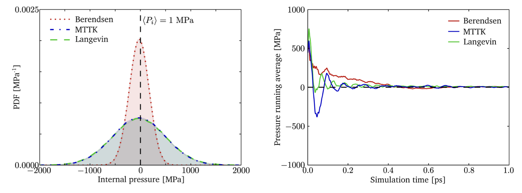
MTTK and Langevin produce identical ensembles, but Langevin barostat oscillates less then MTTK and converges faster due to stochastic collisions and damping.
Reprinted with permission from Rogge et al. 2015, A Comparison of Barostats for the Mechanical Characterization of Metal−Organic Frameworks, J Chem Theory Comput. 2015;11: 5583-97. doi:10.1021/acs.jctc.5b00748. Copyright 2015 American Chemical Society.
Stochastic Cell Rescaling
The stochastic cell rescaling algorithm was developed by Bernetti and Bussi (2020) as an improved version of the Berendsen pressure bath that samples correct volume fluctuations. It adds a stochastic term to the calculation of the rescaling matrix that causes the local pressure fluctuations to be correct for the canonical (NPT) statistical ensemble while retaining the fast first order decay of the pressure deviations from the target pressure.
- Improved version of the Berendsen barostat.
- Adds stochastic term to rescaling matrix.
- Produces correct fluctuations of local pressure for NPT ensemble.
Therefore stochastic cell rescaling can be applied during both equilibration, while the pressure is still far from the target, which would lead to undesired oscillations when using extended system methods like Parrinello-Rahman or MTTK, as well as during production-md (data collection), where it is important to sample from a correct statistical ensemble.
- Pressure converges fast without oscillations.
- Can be used for all stages of MD, including production.
4. Monte-Carlo pressure control.
Recently several efficient Monte Carlo methods have been introduced. Monte Carlo pressure control samples volume fluctuations at a predefined number of steps at a given constant external pressure. It involves generation of a random volume change from a uniform distribution followed by evaluation of the potential energy of the trial system. The volume move is then accepted with the standard Monte-Carlo probability. Virial is not computed by Monte-Carlo methods, so pressure is not available at runtime, and it is also not printed in energy files.
- Recently several efficient Monte Carlo methods have been introduced.
- Sample volume fluctuations at a predefined number of steps at a given constant external pressure.
- Generate a random volume change, evaluate the potential energy. The volume move is then accepted with the standard Monte-Carlo probability.
- Do not compute virial, so pressure is not available at the runtime, and not printed in energy files.
References:
- Molecular dynamics simulations of water and biomolecules with a Monte Carlo constant pressure algorithm
- Constant pressure hybrid Molecular Dynamics–Monte Carlo simulations
Pitfalls
To ensure stability of a simulation volume must be adjusted very slowly with a small increments at each simulations step. Rapid change of the system size may lead to simulation crash. This can occur, for example when pressure coupling is turned on when you begin simulation from a cold start and turn pressure coupling too early in the heating process. In this case, the difference between the target and the real pressure will be large, the program will try to adjust the density too quickly, and bad things (such as SHAKE failures) are likely to happen.
- If the difference between the target and the real pressure is large, the program will try to adjust the density too quickly.
- Rapid change of the system size may lead to simulation crash.
- To ensure stability of a simulation volume must be adjusted very slowly with a small likely
Conclusion
Each barostat or thermostat technique has its own limitations and it is your responsibility to choose the most appropriate method or their combination for the problem of interest.
Selecting barostats in molecular dynamics packages
| Thermostat\MD package | GROMACS | NAMD | AMBER |
|---|---|---|---|
| Berendsen | pcoupl = Berendsen | BerendsenPressure on | barostat = 1 |
| Stoch. cell rescaling | pcoupl = C-rescale | ||
| Langevin | LangevinPiston on | ||
| Monte-Carlo | barostat = 2 | ||
| Parrinello-Rahman | pcoupl = Parrinello-Rahman | ||
| MTTK | pcoupl = MTTK |
Key Points
Water models
Overview
Teaching: 15 min
Exercises: 0 minQuestions
Why do we want to use water in out simulations?
What water models are commonly used?
How to chose a model of water for a simulation?
Objectives
Learn how water molecules are modeled in simulations
Understand how choice of water model can affect a simulation
Introduction
The goal of bio-molecular simulations is the accurate and predictive computer simulation of the physical properties of biological molecules in their aqueous environments. There are two approaches to solvation: a suitable amount of explicit water molecules can be added to prepare a fully solvated simulation system. Alternatively, water can be treated as a continuous medium instead of individual molecules.
Realistic water environment is essential for accurate simulation of biological molecules.
Two approaches to solvation:
- Add explicit water molecules.
- Treat water as a continuous medium instead of individual molecules.
Continuum models
As continuum models do not add any non-bonded interactions to a simulation system, they are significantly faster than explicit solvation. Implicit water models, however, have limitations. They cannot reproduce the microscopic details of the protein–water interface. The conformational ensembles produced by continuum water models differ significantly from those produced by explicit solvent and cannot identify the native state of the protein [Ref]. In particular, salt bridges were over-stabilized, and a higher-than-native alpha helix population was observed. These models are still useful for example for calculation of binding free energies or for flexible protein-protein docking.
- Significantly faster than explicit solvation.
- Cannot reproduce the microscopic details of the protein–water interface.
- Do not produce same conformational ensembles as explicit water (salt bridges are over-stabilized, a higher-than-native alpha helix population).
- Useful for calculation of binding free energies or for flexible protein-protein docking.
Most molecular dynamics simulations are carried out with explicit water molecules.
Explicit models
Most molecular dynamics simulations are carried out with the solute surrounded by a droplet or periodic box of explicit water molecules. In a typical case, water molecules will account for over 80% of the particles in the simulation. Water–water interactions dominate the computational cost of such simulations, so the model used to describe the water needs to be fast as well as accurate.
- Typically water molecules account for over 80% of the particles in the simulation.
- Water–water interactions dominate the computational cost of such simulations.
- The water model needs to be fast and accurate.
Explicit water models are empirical models focused on reproducing a number of bulk properties in a particular phase. For example, some models reproduce well protein hydration energies, while others predict excellent water structure but not so good for hydration free energy. Most importantly, none of water models accurately reproduce all of the key properties of bulk water simultaneously. Simulators can be adversely affected by inaccurate water models in unpredictable ways.
- Explicit water models are empirical models derived to reproduce some bulk properties in a particular phase.
- None of water models accurately reproduce all of the key properties of bulk water.
- Which water model is optimal for the simulation depends on the desired properties of interest.
Therefore, the desired properties of interest must be considered when choosing a water model for a molecular simulation, since this will determine which model is most appropriate.
An early water model.

Water molecules have OH distance of 0.9572 \(\unicode{x212B}\) and HOH angle of 104.52°. Early water models used a rigid geometry closely matching that of actual water molecules. To achieve this O-H and H-H distances are constrained with harmonic potential.
Point charges in classical water models replace electron density distribution. They are meant to reproduce the electrostatic potential of a molecule. Therefore, they are usually derived by fitting to the electrostatic potential around a water molecule. There are some downsides for this approach, which we will discuss later.
- Rigid geometry closely matching actual water molecule.
- O-H and H-H distances are constrained with harmonic potential.
- Point charges replace electron density distribution.
How are water models derived?
A good water model must faithfully reproduce six bulk properties of water:
- Static dielectric constant, \(\epsilon_{0}\)
- Self diffusion coefficient, \(\vec{D}\)
- Heat of vaporization, \(\Delta{H}_{vap}\)
- Isobaric heat capacity, \(\vec{C}_{p}\)
- Thermal expansion coefficient, \(\alpha_{p}\)
- Isothermal compressibility, \(\kappa_{T}\)
Many water models with different level of complexity (the number of interaction points) have been developed. We will discuss only the models most widely used in simulations, and refer you to the excellent article in Wikipedia for an overview of all water models.
3-charge 3-point models.
These models have three interaction points corresponding to the atoms of the water molecule. Only oxygen atom has the Lennard-Jones parameters.
- Three interaction points corresponding to the atoms of the water molecule.
- Only oxygen atom has Lennard-Jones parameters.
- 3-site models are commonly used because computationally they are highly efficient.
| TIP3P (transferable intermolecular potential) $\circ$ Rigid geometry closely matching actual water molecule. |
 |
| SPC/E (simple point charge) $\circ$ More obtuse tetrahedral angle of 109.47°. $\circ$ Adds an average polarization correction to the potential energy function. $\circ$ Reproduces density and diffusion constant better than the original SPC model. |
 |
Models with three sites are commonly used because they are computationally efficient. The interactions between two molecules can be computed using only nine distances.
3-charge 4-point models.
In these models the negative charge is not centered on the oxygen atom, but shifted towards hydrogen atoms. This position is represented with the fourth dummy atom (EP) located near the oxygen along the bisector of the HOH angle. The idea is to improve representation of electrostatic potential without changing its geometric properties. The idea is to improve electrostatic potential representation without changing the geometric properties of the molecule.
- The negative charge is not centered on the oxygen atom, but shifted towards hydrogen atoms
- The position of charge is represented with the fourth dummy atom (EP)
- EP is located near the oxygen along the bisector of the HOH angle.
| TIP4P-Ew $\circ$ Improves association/dissociation balance compared to 3-point models. |
 |
Water models have their limitations.
It is important to understand the limitations of water models. Models are unable to reproduce quantitatively all characteristics of real water. When chosen appropriately for the problem, however, they can provide useful insight into water’s behavior.
- Early water models were developed with cut-off of electrostatic interactions. Using these models with full electrostatic method results in stronger electrostatic interactions and consequently higher density.
- Most of the more complex new water models attempt to reproduce specific properties of a specific phase, but this comes at the expense of other properties.
- TIP3P model predicts hydration free energies of small neutral molecules more accurately than the TIP4PEw model.
- 4-charge 5-point model TIP5P predicts excellent water structure, but poor hydration energies.
Challenges in developing water models.
A key challenge in developing water models is to find an accurate yet simplified description of the charge distribution of the water molecule that can adequately account for the hydrogen bonding in the liquid phase.
Traditional approach is to place point charges on or near the nuclei. Afterwards, however, it was discovered that 3 point charges reproduce the electrostatic potential of water molecules significantly more accurately when they form tight clusters.
- Finding an accurate yet simplified description of the charge distribution that can adequately account for the hydrogen bonding in the liquid phase.
- Traditional approach is to place point charges on or near the nuclei.
- Electrostatic potential of water molecule is reproduced considerably more accurately with 3 point charges when they form tight cluster.
Optimal Point Charges (OPC and OPC3)

The last and the latest water models we will look at is the OPC (Optimal Point Charges). OPC [2] belongs to the family of 3 charge, 4 point models while OPC3 is 3 charge, 3 point version [4]. The key difference from the previous models is that it was designed without geometrical restraints. This design approach is based on the observation that QM electrostatic potential of water molecule is reproduced considerably more accurately with 3 point charges when they form tight cluster of the point charges away from the nuclei than the more traditional distribution with point charges placed on or near the nuclei.
- Removing point charge positioning restrictions allowed for considerably better reproduction of the six bulk properties of water.
- Designed without geometrical restraints.
- Considerably better reproduces the six bulk properties of water.
Polarizable water model OPC3-pol
Rigid models with fixed charges are far from perfect since they do not account for many of the physical effects of real water. Among these physical effects are many subtle quantum effects, water flexibility, and, most importantly, electronic polarizability. In the absence of polarizability, a model cannot respond to changes in polarity in its micro-environment, which is very relevant in many types of simulations. As an example, the dipole moment of a real water molecule changes by almost 40% when it crosses the water-vapor interface, whereas with a fixed charge model, the dipole moment does not change.
Polarization is usually achieved by adding model oscillators, referred to as Drude particles. The Drude particle is a massless virtual site with a partial electric charge attached to an atom by means of a harmonic spring. Simulations of classical Drude oscillator involve repositioning the Drude particle via a computationally expensive self-consistent procedure.
This cost can be reduced by assigning a small mass to each Drude particle, and evolving the simulation using the extended Lagrangian dynamics. Simulations using polarizable water models such as (iAMOEBA and SWM4-NDP) still take at least four times as long as those using rigid non-polarizable water. Additionally, Drude water models have the drawback of requiring matching, polarizable force fields for biomolecules.
OPC3-pol performs almost as well as non-polarizable water models and requires no specialized force fields for proteins or nucleic acids. For high computational efficiency, the OPC3-pol model treats the Drude particle as an “ordinary” atom in the molecular dynamics system: the water oxygen mass is split equally between the oxygen atom and the Drude particle.
The critical benefit of the approach is that OPC3-pol water model can run as fast as classical non-polarizable water models with the existing biomolecular force fields.
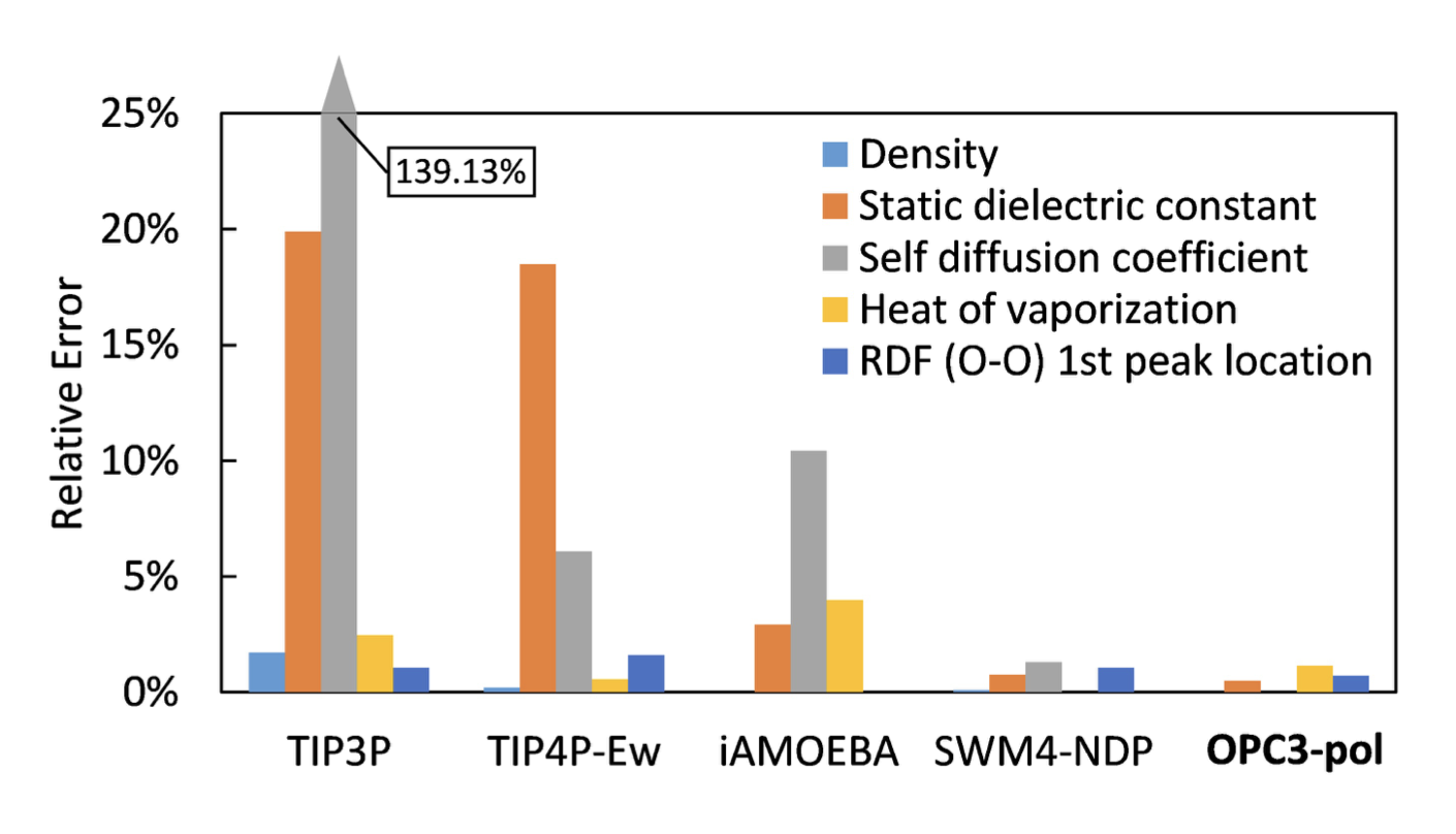
Quality of different water models
Let’s have a look at the quality scores of different water models summarized in the figure below. The figure shows how quality score depends on the dipole and quadrupole moments. Interestingly the test models in which the moments were close to the QM values had low quality. And the models that scored better had moments very different from the QM values.
- The test models in which the moments were close to the QM values had low quality.
- The models that scored better had moments very different from the QM moments.
This indicates that three point charges, even if placed optimally, are not enough to represent the complex charge distribution of real water molecule to the needed degree of accuracy.
The distribution of quality scores for different water models in the space of dipole (μ) and quadruple (QT) moments. Figures from [2].
Performance Considerations
The time to compute interactions between a pair of water molecules is approximately proportional to the number of distances between each pair of interaction points. For the 3-point model, 9 distances are required for each pair of water molecules. For the 4-site model, 10 distances are required (every charged site with every charged site, plus the VDW O–O interaction).
- Computation cost is proportional to the number of pairwise distances.
- 3-charge 3-point model: 9 distances
- 3-charge 4-site model: 10 distances (3x3 Coulomb interactions plus one VDW O–O interaction).
Other things to consider
Water models in common use in bio-molecular simulation have traditionally only been parameterized for a single temperature of 298K (SPC/E, TIP3P, etc.)
Force Field Parameters of the common Water Models
| TIP3P | SPC/E | TIP4P-Ew | OPC | OPC3 | |
|---|---|---|---|---|---|
| OH | 0.9572 | 1.0 | 0.9572 | 0.8724 | 0.9789 |
| HH | 1.5136 | 1.63 | 1.5136 | 1.3712 | 1.5985 |
| HOH | 104.52 | 109.47 | 104.52 | 103.6 | 109.47 |
| OM | - | - | 0.125 | 0.1594 | - |
| A(12) | 582.0 | 629.4 | 656.1 | 865.1 | 667.9 |
| B(6) | 595.0 | 625.5 | 653.5 | 858.1 | |
| qO | −0.834 | −0.8476 | −1.04844 | −1.3582 | -0.8952 |
| qH | +0.417 | +0.4238 | +0.52422 | +0.6791 | +0.4476 |
Nonbonded OPC3: sigma=1.7814990, epsilon=0.163406 pending convert to A, B
- Structure and Dynamics of the TIP3P, SPC, and SPC/E Water Models at 298 K
- Building Water Models: A Different Approach
- Effect of the Water Model in Simulations of Protein–Protein Recognition and Association
- Accuracy limit of rigid 3-point water models
- A fast polarizable water model for atomistic simulations
Key Points
Continuum models cannot reproduce the microscopic details of the protein–water interface
Water–water interactions dominate the computational cost of simulations
Good water model needs to be fast and accurate in reproduction of the bulk properties of water
End of Workshop
Overview
Teaching: min
Exercises: minQuestions
Objectives
Key Points
Supplemental: Overview of the Common Force Fields
Overview
Teaching: 0 min
Exercises: 0 minQuestions
What are the categories of molecular dynamics force fields?
What force fields are available?
What systems they work best with?
Objectives
Be able to recognize the strengths and weaknesses of different types of force fields.
Find out which force fields are available and which systems they are most suitable for.
Identify the original papers that introduced force fields.
- Early Force Fields
- Evolution of Force Fields
- Force Fields Aimed at Improving Quality of Molecular Interactions
- CVFF (Consistent Valence Force Field) (Maple & Hagler, 1988)
- CFF93 (An ab initio all-atom force field for polycarbonates) (Sun et al., 1994)
- CFF, formerly CFF95 (Jonsdottir & Rasmussen, 2000)
- MM3 (N.L.Allinger et al., 1989), MM4 (N.L.Allinger et al., 1996)
- COMPASS (Condensed-phase Optimized Molecular Potentials for Atomistic Simulation Studies)
- Biomolecular Force Fields for Large-Scale Simulations.
- Polarizable Force fields
- Force Fields for Small Molecules
- Additional Reading
Early Force Fields
CFF (Consistent Force Field) (1968)
CFF was the first modern force field (Lifson, 1968) Introduced a concept of a ‘consistent force field’. Introduced a methodology for deriving and validating force fields. The term ‘consistent’ emphasized importance of the ability to describe a wide range of compounds and physical observables (conformation, crystal structure, thermodynamic properties and vibrational spectra). After the initial derivation for hydrocarbons CFF was extended to proteins, but was very crude at that time.
Allinger Force Fields (MM1 - MM4) (1976-1996)
- MM1 (N.L. Allinger, 1976) - Class 1
- MM2 (N.L. Allinger, 1977) - Class 1
- MM3 N.L.Allinger et al., 1989 - Class 2
- MM4 (N.L.Allinger et al., 1996) - Class 3
Target data included electron diffraction, vibrational spectra, heats of formation, and crystal structures. The calculation results were verified via comparison with high-level ab-initio quantum chemistry computations, and the parameters were additionally adjusted. Intended for calculations on small and medium size organic molecules.
ECEPP (Empirical Conformational Energy Program for Peptides) (1975)
ECEPP was the first force field targeting polypeptides and proteins. Crystal data of small organic compounds and semi-empirical QM calculations were used extensively in derivation of this force field. As more experimental data became available, force field parameters have been refined and modified versions were published.
- ECEPP (F. A. Momany, et al., 1975)
- UNICEPP (L.G. Dunfield, 1978) The united atoms version of ECEPP, developed for the conformational analysis of large molecules
- ECEPP-02 (G. Nemethy et al, 1983)
- ECEPP-03 (G. Nemethy et al, 1992)
- ECEPP-05 (Y. A. Arnautova et al., 2006)
Evolution of Force Fields
Early force field advances
Early force field development focused on developing mathematical forms for MM energy function and methods of deriving parameters. Researchers investigated various forms of potential energy functions, and experimented with hydrogen bonding potential, combination rules, and out of plane angle potentials during this period.
United atoms force fields.
United Atoms Model was developed to speed up large-scale simulations. It represents nonpolar carbons and their bonded hydrogens as a single particle. United Atoms force fields can significantly reduce the size of most simulations, since roughly half of the atoms in biological or other organic macromolecules are hydrogens. Additional advantage is the efficiency gain in conformational sampling. The first united atoms force field was UNICEPP (L.G. Dunfield, 1978).
According to early comparisons between all-atom and united-atom simulations, united-atom force fields adequately represent molecular vibrations and bulk properties of small molecules.
After this initial success all major developers of protein force fields implemented united atoms models:
It became apparent, however, that there were some limitations:
- In the absence of explicit hydrogens, hydrogen bonds cannot be accurately treated;
- π-stacking cannot be represented without explicitly including hydrogens in aromatic groups;
- when hydrogens were combined with polar heavy atoms, dipole and quadrupole moments were found to be inaccurate.
New approaches were found to overcome the limitations of united-atom force fields. For example, only aliphatic hydrogens, which are not significantly charged and do not participate in hydrogen bonds, are represented as united atoms while other hydrogens are represented explicitly. In this way, the limitations of the united-atom force field are partially mitigated while preserving most of the benefits of the united-atom force field.
Refinement after the initial introduction.
Statistical errors caused by relatively short simulation lengths and systematic errors caused by inaccurate force fields limit the predictive power of MD simulations. Deficiencies of the force fields remained undetected when statistical errors caused by insufficient sampling prevailed. Increase of the computing power over last two decades allowed for much longer simulations and resulted in a significant reduction of statistical errors. This led to the detection of force field deficiencies such as large deviations in different observables and inability to predict conformations of proteins and peptides. Various approaches were undertaken to improve force fields such as:
-
Use an all-atom model to increase accuracy. Most force fields (CHARMM22, AMBER ff99 and GAFF, OPLS-AA, OPLS-AA/L) converted back to all-atom model.
-
Increase the size of the target data. Because each force field was derived with a different training set of atomic configurations, it was biased in one way or another. By using large atomic reference sets and careful selection of the atomic configurations, bias problems were reduced and accuracy was improved.
- Improve representation of static electrostatic potential. The atom-centered point charge model has two shortcomings:
- It is unable to describe the anisotropy of the charge distribution;
- It does not account for the charge penetration effect (deviation of electrostatic interaction from the Coulomb form due to electron shielding when atomic electron clouds overlap).
In molecular complexes, these effects determine equilibrium geometry and energy. Examples of anisotropic charge distribution are σ-holes, lone pairs, and aromatic systems.
In covalent bonding an atom’s side opposite its bond usually has a lower electron density region known as σ-hole. Through a positive electrostatic potential associated with a sigma-hole, an atom can interact attractively with negative sites.
A simple solution to the σ-hole model is to attach an off-centered positive charge to the halogen atom ( W. Jorgensen & P. Schyman, 2012, F.Lin, A. MacKerell, 2018). An atomic multipole method provides a more thorough way of describing anisotropic charge distribution (J.Ponder et al., 2010).
- Include polarization effects. Early force fields employed fixed atomic charges to model the electrostatic interactions. Fixed-charge electrostatics does not account for the many-body polarization that can vary significantly depending on chemical and physical environments. Consequently, non-polarizable force fields fail to capture the conformational dependence of electrostatic properties. Polarizable force fields where the charges can be calculated from the energy equilibration have been developed ot address this problem (see a recent review). A drawback of including polarization is that simulations take longer to run due to the high computational cost.
Recent developments in force fields and future prospects
Despite extensive attempts to improve force files, they have often failed to achieve quantitative accuracy. There was a realization that the functional form of potential energy was the major problem with all widely used protein force fields.
Two strategies can be used to address this problem:
- Expand and improve the rigor of the representation of the underlying physics.
- Develop empirical corrections to compensate for deficiency of physical representation
AMBER, CHARMM, and OPLS focused their efforts on empirical correction of the simple potential function. AMOEBA and COMPASS worked on improving the functional form.
It is well understood that charge distributions are affected by both chemical environments and local geometry changes. As we discussed above, the former is explicitly treated in polarizable force field models. AMOEBA+ (2019) improved representation of electrostatic interactions by incorporating charge penetration and intermolecular charge transfer.
Dependence of atomic charges on the local molecular geometry is ignored by almost all classical force fields even though it is well known that it causes issues.
One of the few force fields that consider CF contributions is SDFF:
https://eurekamag.com/research/011/176/011176666.php
Palmo, K.; Mannfors, B.; Mirkin, N. G.; Krimm, S. Inclusion of charge and polarizability fluxes provides needed physical accuracy in molecular mechanics force fields. Chem. Phys. Lett. 2006, 429 (4), 628.
Recently Geometry-Dependent Charge Flux (GDCF) model considering charge flux contributions along bond and angle was introduced in AMOEBA+(CF) force field.
Implementation of Geometry-Dependent Charge Flux into the Polarizable AMOEBA+ Potential
Force Fields Aimed at Improving Quality of Molecular Interactions
CVFF (Consistent Valence Force Field) (Maple & Hagler, 1988)
CFF93 (An ab initio all-atom force field for polycarbonates) (Sun et al., 1994)
CFF, formerly CFF95 (Jonsdottir & Rasmussen, 2000)
MM3 (N.L.Allinger et al., 1989), MM4 (N.L.Allinger et al., 1996)
COMPASS (Condensed-phase Optimized Molecular Potentials for Atomistic Simulation Studies)
COMPASS (H. Sun, 1998)
Developed for simulations of organic molecules, inorganic small molecules, and polymers
COMPASS II (H. Sun et al., 2016)
Extended the coverage to polymer and drug-like molecules found in popular databases. The VDW parameters are obtained by fitting enthalpies of vaporization and densities, to experimental data. The atomic partial charges are derived using QM and empirically adjusted to take hydrogen bonding effects into account. The COMPASS energy function offers six types of cross-terms: bond-bond, bond-angle, angle-angle, bond-torsion, angle-torsion, and angle-torsion-angle.
Biomolecular Force Fields for Large-Scale Simulations.
Long simulations of large systems are required to study biologically relevant processes. It takes a lot of computer power to run such simulations. Due to this, the main objective is to develop a minimal force field that allows simulation sizes and time periods to be extended as much as possible while still keeping chemical structures, interaction energies, and thermodynamic properties within an acceptable range.
The workhorses of modern biomolecular simulations are all-atom, fixed-charge force fields:
- AMBER (Assisted Model Building with Energy Refinement)
- CHARMM (Chemistry at HARvard Macromolecular Mechanics)
- GROMOS (GROningen MOlecular Simulation)
- OPLS (Optimized Potentials for Liquid Simulations)
CHARMM and AMBER forcefields are developed for simulations of proteins and nucleic acids, and they focus on accurate description of structures and non-bonded energies. GROMOS and OPLS are geared toward accurate description of thermodynamic properties such as heats of vaporization, liquid densities, and molecular solvation properties.
AMBER
AMBER forcefields are developed for simulations of proteins and nucleic acids and they are focused on accurate description of structures and non-bonded energies. The VDW parameters are obtained from crystal structures and lattice energies. The atomic partial charges are fitted to QM electrostatic potential without any empirical adjustments.
ff99 (1999)
The main idea is that the use of RESP charges, should lead to the need for fewer torsional potentials than in models with an empirical charge derivation. Potential energy surface scans were performed using four different ab initio methods, HF/6‐31G*, MP2/6‐31G*, MP2/6‐311+G (2d,p), and B3LYP/6‐311+G (2d,p).
Wang J, Cieplak P, Kollman PA. How well does a restrained electrostatic potential (RESP) model perform in calculating conformational energies of organic and biological molecules? Journal of Computational Chemistry. 2000;21: 1049–1074. doi:10.1002/1096-987X(200009)21:12<1049::AID-JCC3>3.0.CO;2-F
After publication of ff99 a number of studies devoted primarily to modifying the torsion potentials in order to correct the observed discrepancies have been published:
ff03 (2003)
Completely new charge set developed using B3LYP/cc-pvTZ quantum calculations in a polarizable continuum (PCM) solvent intended to mimic the interior of a protein. Backbone torsion Fourier series were derived specifically for this new charge set at the MP2/cc-pvTZ level of theory, also in the context of PCM solvent. MM gas-phase energies computed with charges derived in PCM solvent have been shown to double-count polarization effects, and ff03 force field has not become as widely used or further refined as ff99
Duan, Yong, Chun Wu, Shibasish Chowdhury, Mathew C. Lee, Guoming Xiong, Wei Zhang, Rong Yang, et al. “A point-charge force field for molecular mechanics simulations of proteins based on condensed-phase quantum mechanical calculations.” Journal of Computational Chemistry 24, no. 16 (2003): 1999–2012. https://doi.org/10.1002/jcc.10349.
ff99sb (2006)
Optimized for the correct description of the helix-coil equilibrium
ff99SB-φ’
Targeted the reproduction of the intrinsic conformational preferences of tripeptides
ff99SBnmr (2010) and ff99SB_φψ
Target data included protein NMR chemical shifts and residual dipolar couplings.
ff99SBildn (2010)
Targeted optimization of four amino acid side chains.
Lindorff‐Larsen, Kresten, Stefano Piana, Kim Palmo, Paul Maragakis, John L. Klepeis, Ron O. Dror, and David E. Shaw. “Improved Side-Chain Torsion Potentials for the Amber Ff99SB Protein Force Field.” Proteins: Structure, Function, and Bioinformatics 78, no. 8 (2010): 1950–58. doi:10.1002/prot.22711.
ff12SB (2012)
This is the preliminary version of ff14SB described in the same paper.
ff12SB-cMAP (2015)
Force field for implicit-solvent simulations.
ff99IDPs (2015)
Force field for intrinsically disordered proteins
ff14ipq (2014)
This force field is derived using another new approach aiming to derive charges implicitly polarized by the fixed charge explicit water (IPolQ method). The charges are derived in self-consistent manner in presence of explicit water molecules represented by TIP4P-Ew water model at MP2/cc-pV(T+d)Z level. The weak point of the ff14ipq force field is overstabilization of salt bridges.
Cerutti, David S., William C. Swope, Julia E. Rice, and David A. Case. Ff14ipq: A Self-Consistent Force Field for Condensed-Phase Simulations of Proteins. Journal of Chemical Theory and Computation 10, no. 10 (October 14, 2014): 4515–34. doi:10.1021/ct500643c.
ff14SB (2015)
Another attempt to corect for deficiencies of ff99SB by using new side chain dihedral parameters based on MP2 level calculations followed by adjustment to the backbone φ energy profile. Used the old ff99SB charge set.
Maier, James A., Carmenza Martinez, Koushik Kasavajhala, Lauren Wickstrom, Kevin E. Hauser, and Carlos Simmerling. “Ff14SB: Improving the Accuracy of Protein Side Chain and Backbone Parameters from Ff99SB.” Journal of Chemical Theory and Computation 11, no. 8 (August 11, 2015): 3696–3713. https://doi.org/10.1021/acs.jctc.5b00255.
ff15ipq (2016)
The motivation for the development was to address the salt bridge overstabilization problem of ff14ipq. However, this forcefiled is not a small correction applied to ff14ipq. It is is a complete semi-automatic rederivation of all parameters with the different water model SPC/Eb. The salt bridge overstabilization issue was addressed by increasing radius of polar hydrogens bonded to nitrogen. The modified FF performed as well or better than the other fixed charge force fields. Polarizable CHARMM Drude-2013 and AMOEBA performed better in this respect, as expected.
Problems related to protein stability persist. Even 4 μs simulations “were not sufficiently long to obtain converged estimates of secondary structure of polypeptides”. In simulation tests some proteins deviated significantly near the end of several microsecond simulations, and it is not clear whether this is a transient fluctuation or transition to a different state.
Debiec, Karl T., David S. Cerutti, Lewis R. Baker, Angela M. Gronenborn, David A. Case, and Lillian T. Chong. Further along the Road Less Traveled: AMBER Ff15ipq, an Original Protein Force Field Built on a Self-Consistent Physical Model. Journal of Chemical Theory and Computation 12, no. 8 (August 9, 2016): 3926–47. doi:10.1021/acs.jctc.6b00567
ff15FB (2017)
The goal was to reoptimize intramolecular bond, angle, and dihedral parameters to fit MP2 level QM data without modifying the nonbonded parameters. The parameter optimization was done using ForceBalance package. Same peformance as the earlier versions for equilibrium properties, improved performance for temperature dependence. For best agreement with experiment recommended to use with the TIP3P-FB water. The TIP3P-FB model was parametrized to reproduce the temperature and pressure dependence of a wide range of thermodynamic properties.
ff19SB (2020)
Backbone dihedral parameters optimized using as reference data the entire 2D quantum mechanics (QM) energy surface. Both QM and MM calculations were done in aqueous solution. AMBER ff19SB uses CMAP torsional potentials. The authors concluded that “ff19SB, when combined with a more accurate water model such as OPC, should have better predictive power for modeling sequence-specific behavior, protein mutations, and also rational protein design”.
CHARMM
CHARMM19 (1996)
United-atom model, originally released in 1985.
CHARMM22 (1998)
All-atom model.
CHARMM27 (2000)
Update to the CHARMM22 featuring the optimization of nucleic acid and lipid parameters, as well as the introduction of a number of new ions.
CHARMM22/CMAP (2004)
This forcefield introduces a tabulated correction for the φ-, ψ-angular dependence of the potential energy. As a result of the application of CMAP correction, the dynamical and structural properties of proteins were significantly improved in molecular dynamics simulations.
CHARMM27r (2005)
Improved lipid parameter set.
CHARMM35 (2008)
Carbohydrate parameter set.
CGenFF (2009)
CHARMM36 (2012)
refined backbone CMAP potentials and introduced new side-chain dihedral parameters. The updated CMAP corrected the C22/CMAP FF bias towards alpha-helical conformations.
Review
CHARMM Force Field Files
GROMOS
53A5, 53A6 (Oostenbrink et al., 2004)
54A7, 54B7 (N.Schmid et al., 2011)
54A8 (M.M.Reif et al., 2012)
Parameter sets for GROMOS force fields are specified in accordance with the following format:
- The number of atom types
- A letter code that describes for what conditions the parameters are optimized (e.g. A - solution, B - vacuum).
- The version number
OPLS
Force fields of the OPLS family are designed for simulating liquids that contain organic molecules and proteins. The VDW parameters are optimized using experimental liquid properties, mainly enthalpies of vaporization and densities. The atomic partial charges are derived using QM and experimental condensed-phase properties. An important part of the OPLS philosophy is balancing solvent-solvent and solute-solvent interactions.
OPLS-AA (1996)
This is the first all-atom OPLS force field. Bond stretching and angle bending parameters are taken from the AMBER force field. The torsional parameters were fit to the RHF/6-31G* calculations of about 50 organic molecules and ions. The charges are empirical and have been obtained from fitting to reproduce properties of organic liquids.
Jorgensen W, Maxwell D, Tirado-Rives J. Development and testing of the OPLS all-atom force field on conformational energetics and properties of organic liquids. J Am Chem Soc. 1996;118: 11225–11236.
OPLS-AA/L (2001)
Large data set, more than 2000 data points of energies for the 20 amino acids based on geometry optimization at the HF/6-31G** level followed by single-point LMP2/cc-pVTZ(-f) calculations. This level of theory is accurate within 0.25 kcal/mol.
Kaminski GA, Friesner RA, Tirado-Rives J, Jorgensen WL. Evaluation and Reparametrization of the OPLS-AA Force Field for Proteins via Comparison with Accurate Quantum Chemical Calculations on Peptides. J Phys Chem B. 2001;105: 6474–6487. doi:10.1021/jp003919d
OPLS_2005 (2005)
Main goal - to broaden the coverage of OPLS_2001 and refine torsion parameters using a larger dataset. The new Data set included torsion profiles from 637 compounds.
Banks JL, Beard HS, Cao Y, Cho AE, Damm W, Farid R, et al. Integrated Modeling Program, Applied Chemical Theory (IMPACT). J Comput Chem. 2005;26: 1752–1780. doi:10.1002/jcc.20292
OPLS-AAx & OPLS/CM1Ax (2012)
The representation of chlorine, bromine, and iodine in aryl halides has been modified in the OPLS-AA and OPLS/CM1A force fields in order to incorporate halogen bonding. It was accomplished by adding a partial positive charge in the region of the σ-hole.
OPLS2.0 (2012)
OPLS2 was developed to improve the accuracy of drug-like molecules. Substantially expanded data set contained QM data on more than 11,000 molecules. CM1A-BCC charges were used. The BCC terms were parameterized against the OPLS-AA charges for a core set of 112 molecules and the electrostatic potential at the HF/6-31G* level. The BCC terms were empirically adjusted to minimize the errors with regard to the ASFE using a training set of 153 molecules.
Shivakumar D, Harder E, Damm W, Friesner RA, Sherman W. Improving the Prediction of Absolute Solvation Free Energies Using the Next Generation OPLS Force Field. J Chem Theory Comput. 2012;8: 2553–2558. doi:10.1021/ct300203w
OPLS-AA/M (2015)
New torsion parameters using higher level ωB97X-D(23)/6-311++G(d,p) and B2PLYP-D3BJ/aug-cc-pVTZ(26) QM calculations.
Robertson MJ, Tirado-Rives J, Jorgensen WL. Improved Peptide and Protein Torsional Energetics with the OPLS-AA Force Field. J Chem Theory Comput. 2015;11: 3499–3509. doi:10.1021/acs.jctc.5b00356
OPLS3 (2016)
Added off-atom charge sites to represent halogen bonding and aryl nitrogen lone pairs. Complete refit of peptide dihedral parameters using an order of magnitude more data. Claimed 30% improvement. Still the same original VDW parameters.
Harder E, Damm W, Maple J, Wu C, Reboul M, Xiang JY, et al. OPLS3: A Force Field Providing Broad Coverage of Drug-like Small Molecules and Proteins. J Chem Theory Comput. 2016;12: 281–296. doi:10.1021/acs.jctc.5b00864
Polarizable Force fields
AMBER
ff02pol (P. Cieplak et al., 2001)
ff12pol (J. Wang et al., 2011)
AMOEBA (Atomic Multipole Optimized Energetics for Biomolecular Applications)
AMOEBA-2002 (Ren and Ponder, 2002)
AMOEBA-2013 (Shi et al., 2013)
AMOEBA-2013 uses permanent electrostatic multipole (dipole and quadrupole) moments at each atom and explicitly treats polarization effects under various chemical and physical conditions.
AMOEBA+ (C. Liu et al., 2019)
AMOEBA+(CF) (C. Liu et al., 2020)
Q-AMOEBA (N.Mauger et al., 2022)
OPLS
OPLS/PFF https://onlinelibrary.wiley.com/doi/10.1002/jcc.10125
Force field for water with polarization capabilities. Intended for simulations that explicitly take nuclear quantum effects into account.
CHARMM
CHARMM fluctuating charge model (S.Patel et al., 2004)
CHARMM Drude model (P.E.M. Lopez, 2013)
Force Fields for Small Molecules
GAFF
CGenFF
- (F.-U.Lin & AD. MacKerell, 2020) Force Fields for Small Molecules
Additional Reading
-
(Dauber-Osguthorpe, 2019) Biomolecular force fields: where have we been, where are we now, where do we need to go and how do we get there? - Review of the origins of FF based calculations, theory and methodology of FF development.
-
(Hagler, 2019) Force field development phase II: Relaxation of physics-based criteria… or inclusion of more rigorous physics into the representation of molecular energetics. - The latest developments in improvement of FF accuracy and robustness are discussed.
-
Tinker-HP is a multi-CPUs and multi-GPUs/multi-precision, MPI massively parallel package dedicated to long molecular dynamics simulations with classical and polarizable force fields, neural networks and advanced QM/MM.
Key Points
There are different types of force fields designed for different types of simulations.
Induction effects are not accounted for by fixed-charge force fields.
Using more accurate and diverse target data allows MD force fields to be improved.