Force Fields and Interactions
Overview
Teaching: 30 min
Exercises: 0 minQuestions
What is Molecular Dynamics and how can I benefit from using it?
What is a force field?
What mathematical energy terms are used in biomolecular force fields?
Objectives
Understand strengths and weaknesses of MD simulations
Understand how the interactions between particles in a molecular dynamics simulation are modeled
Introduction
Atoms and molecules, the building blocks of matter, interact with each other. They are attracted at long distances, but at short distances the interactions become strongly repulsive. As a matter of fact, there is no need to look for a proof that such interactions exist. Every day, we observe indirect results of these interactions with our own eyes. For example, because of the attraction between water molecules, they stick together to form drops, which then rain down to fill rivers. On the other hand, due to the strong repulsion, one liter of the same water always weighs about 1 kg, regardless of how much pressure we use to compress it.
Nowadays, molecular modeling is done by analyzing dynamic structural models in computers. Historically, the modeling of molecules started long before the invention of computers. In the mid-1800’s structural models were suggested for molecules to explain their chemical and physical properties. First attempts at modeling interacting molecules were made by van der Waals in his pioneering work “About the continuity of the gas and liquid state” published in 1873. A simple equation representing molecules as spheres that are attracted to each other enabled him to predict the transition from gas to liquid. Modern molecular modeling and simulation still rely on many of the concepts developed over a century ago. Recently, MD simulations have been vastly improved in size and length. With longer simulations, we are able to study a broader range of problems under a wider range of conditions.
- Atoms and molecules interact with each other.
- We carry out molecular modeling by following and analyzing dynamic structural models in computers.
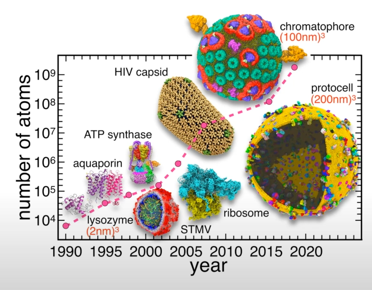 Figure from: AI-Driven Multiscale Simulations Illuminate Mechanisms of SARS-CoV-2 Spike Dynamics
- The size and the length of MD simulations has been recently vastly improved.
- Longer and larger simulations allow us to tackle wider range of problems under a wide variety of conditions.
Recent example - simulation of the whole SARS-CoV-2 virion
One of the recent examples is simulation of the whole SARS-CoV-2 virion. The goal of this work was to understand how this virus infects cells. As a result of MD simulations, conformational transitions of the spike protein as well as its interactions with ACE2 receptors were identified. According to the simulation, the receptor binding domain of the spike protein, which is concealed from antibodies by polysaccharides, undergoes conformational transitions that allow it to emerge from the glycan shield and bind to the angiotensin-converting enzyme (ACE2) receptor in host cells.
The virion model included 305 million atoms, it had a lipid envelope of 75 nm in diameter with a full virion diameter of 120 nm. The multiscale simulations were performed using a combination of NAMD, VMD, AMBER. State-of-the-art methods such as the Weighted Ensemble Simulation Toolkit and ML were used. The whole system was simulated on the Summit supercomputer at Oak Ridge National Laboratory for a total time of 84 ns using NAMD. In addition a weighted ensemble of a smaller spike protein systems was simulated using GPU accelerated AMBER software.
This is one of the first works to explore how machine learning can be applied to MD studies. Using a machine learning algorithm trained on thousands of MD trajectory examples, conformational sampling was intelligently accelerated. As a result of applying machine learning techniques, it was possible to identify pathways of conformational transitions between active and inactive states of spike proteins.
- System size: 304,780,149 atoms, 350 Å × 350 Å lipid bilayer, simulation time 84 ns
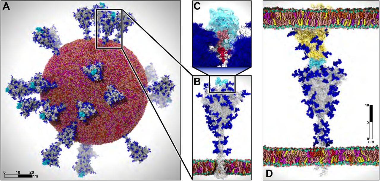 Figure from AI-Driven Multiscale Simulations Illuminate Mechanisms of SARS-CoV-2 Spike Dynamics
- Showed that spike glycans can modulate the infectivity of the virus.
- Characterized interactions between the spike and the human ACE2 receptor.
- Used ML to identify conformational transitions between states and accelerate conformational sampling.
Goals
In this workshop, you will learn about molecular dynamics simulations and how to use different molecular dynamics simulation packages and utilities, such as NAMD, VMD, and AMBER. We will show you how to use Digital Research Alliance of Canada (Alliance) clusters for all steps of preparing the system, performing MD and analyzing the data. The emphasis will be on reproducibility and automation through scripting and batch processing.
- Introduce you to the method of molecular dynamics simulations.
- Guide you to using various molecular dynamics simulation packages and utilities.
- Teach how to use Digital Research Alliance of Canada (Alliance) clusters for system preparation, simulation and trajectory analysis.
The goal of this first lesson is to provide an overview of the theoretical foundation of molecular dynamics. As a result of this lesson, you will gain a deeper understanding of how particle interactions are modeled and how molecular dynamics are simulated.
The focus will be on reproducibility and automation by introducing scripting and batch processing.
The theory behind the method of MD.
Force Fields
The development of molecular dynamics was largely motivated by the desire to understand complex biological phenomena at the molecular level. To gain a deeper understanding of such processes, it was necessary to simulate large systems over a long period of time.
While the physical background of intermolecular interactions is known, there is a very complex mixture of quantum mechanical forces acting at a close distance. The forces between atoms and molecules arise from dynamic interactions between numerous electrons orbiting atoms. Since the interactions between electron clouds are so complex, they cannot be described analytically, nor can they be calculated numerically fast enough to enable a dynamic simulation on a relevant scale.
In order for molecular dynamics simulations to be feasible, it was necessary to be able to evaluate molecular interactions very quickly. To achieve this goal molecular interactions in molecular dynamics are approximated with a simple empirical potential energy function.
- Understanding complex biological phenomena requires simulations of large systems for a long time windows.
- The forces acting between atoms and molecules are very complex.
- Very fast method of evaluations molecular interactions is needed to achieve these goals.
Interactions are approximated with a simple empirical potential energy function.
The potential energy function U is a cornerstone of the MD simulations because it allows calculating forces. A force on an object is equal to the negative of the derivative of the potential energy function:
$\vec{F}=-\nabla{U}(\vec{r})$
Once we know forces acting on an object we can calculate how its position changes in time. To advance a simulation in time molecular dynamics applies classical Newton’s equation of motion stating that the rate of change of momentum \(\vec{p}\) of an object equals the force \(\vec{F}\) acting on it:
$ \vec{F}=\frac{d\vec{p}}{dt} $
To summarize, if we are able to determine a system’s potential energy, we can also determine the forces acting between the particles as well as how their positions change over time. In other words, we need to know the interaction potential for the particles in the system to calculate forces acting on atoms and advance a simulation.
- The potential energy function allows calculating forces: $ \vec{F}=-\nabla{U}(\vec{r}) $
- With the knowledge of the forces acting on an object, we can calculate how the position of that object changes over time: $ \vec{F}=\frac{d\vec{p}}{dt} $.
- Advance system with very small time steps assuming the velocities don’t change.
Let’s examine a typical workflow for simulations of molecular dynamics.
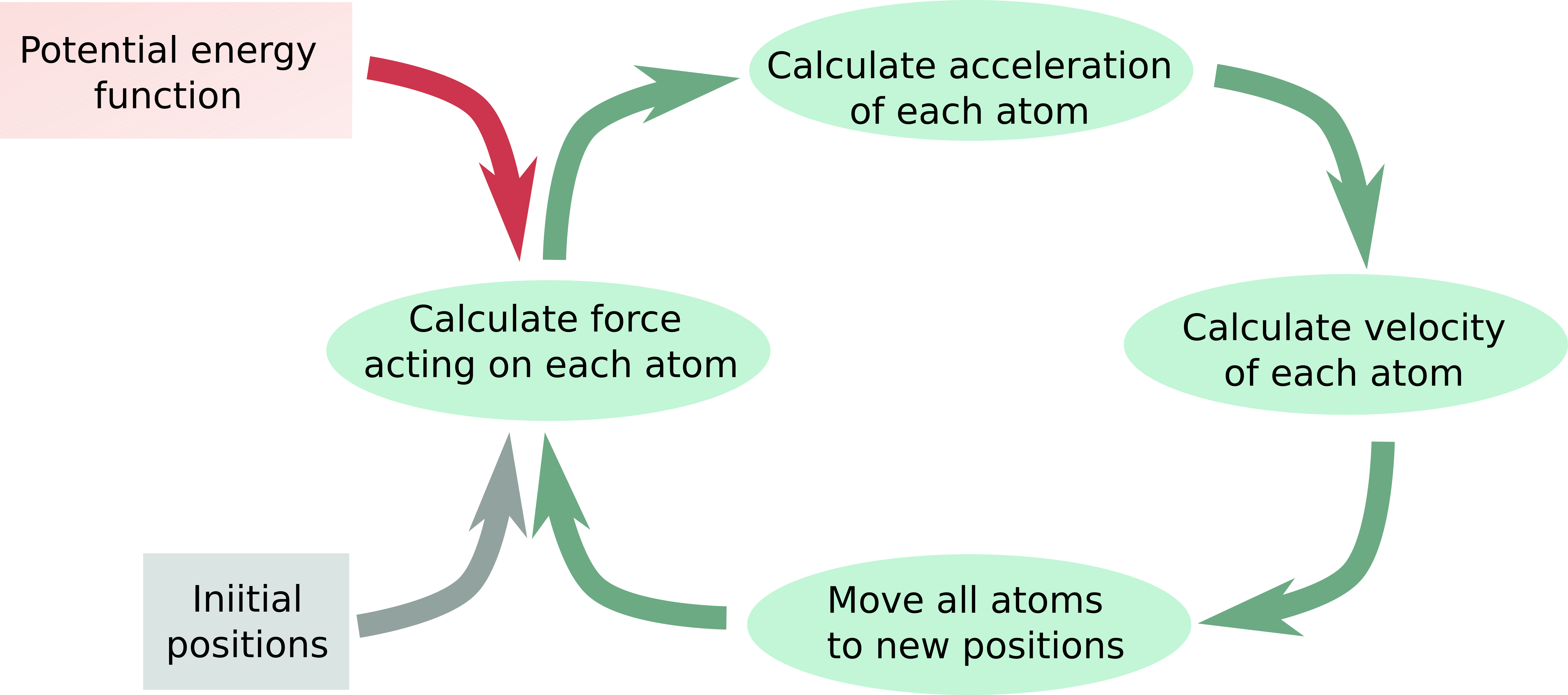 Flow diagram of MD simulation
A force field is a set of empirical energy functions and parameters used to calculate the potential energy U as a function of the molecular coordinates.
Molecular dynamics programs use force fields to run simulations. A force field (FF) is a set of empirical energy functions and parameters allowing to calculate the potential energy U of a system of atoms and/or molecules as a function of the molecular coordinates. Classical molecular mechanics potential energy function used in MD simulations is an empirical function composed of non-bonded and bonded interactions:
- Potential energy function used in MD simulations is composed of non-bonded and bonded interactions:
$U(\vec{r})=\sum{U_{bonded}}(\vec{r})+\sum{U_{non-bonded}}(\vec{r})$
Typically MD simulations are limited to evaluating only interactions between pairs of atoms. In this approximation force fields are based on two-body potentials, and the energy of the whole system is described by the 2-dimensional force matrix of the pairwise interactions.
- Only pairwise interactions are considered.
Classification of force fields.
For convenience force fields can be divided into 3 general classes based on how complex they are.
Class 1 force fields.
In the class 1 force field dynamics of bond stretching and angle bending are described by simple harmonic motion, i.e. the magnitude of restoring force is assumed to be proportional to the displacement from the equilibrium position. As the energy of a harmonic oscillator is proportional to the square of the displacement, this approximation is called quadratic. In general, bond stretching and angle bending are close to harmonic only near the equilibrium. Higher-order anharmonic energy terms are required for a more accurate description of molecular motions. In the class 1 force field force matrix is diagonal because correlations between bond stretching and angle bending are omitted.
- Dynamics of bond stretching and angle bending is described by simple harmonic motion (quadratic approximation)
- Correlations between bond stretching and angle bending are omitted.
Examples: AMBER, CHARMM, GROMOS, OPLS
Class 2 force fields.
Class 2 force fields add anharmonic cubic and/or quartic terms to the potential energy for bonds and angles. Besides, they contain cross-terms describing the coupling between adjacent bonds, angles and dihedrals. Higher-order terms and cross terms allow for a better description of interactions resulting in a more accurate reproduction of bond and angle vibrations. However, much more target data is needed for the determination of these additional parameters.
- Add anharmonic cubic and/or quartic terms to the potential energy for bonds and angles.
- Contain cross-terms describing the coupling between adjacent bonds, angles and dihedrals.
Class 3 force fields.
Class 3 force fields explicitly add special effects of organic chemistry. For example polarization, stereoelectronic effects, electronegativity effect, Jahn–Teller effect, etc.
- Explicitly add special effects of organic chemistry such as polarization, stereoelectronic effects, electronegativity effect, Jahn–Teller effect, etc.
Examples of class 3 force fields are: AMOEBA, DRUDE
Energy Terms of Biomolecular Force Fields
What types of energy terms are used in Biomolecular Force Fields? For biomolecular simulations, most force fields are minimalistic class 1 force fields that trade off physical accuracy for the ability to simulate large systems for a long time. As we have already learned, potential energy function is composed of non-bonded and bonded interactions. Let’s have a closer look at these energy terms.
Non-Bonded Terms
The non-bonded potential terms describe non-electrostatic and electrostatic interactions between all pairs of atoms.
- Describe non-elecrostatic and electrostatic interactions between all pairs of atoms.

Non-electrostatic potential energy is most commonly described with the Lennard-Jones potential.
- Non-elecrostatic potential energy is most commonly described with the Lennard-Jones potential.
The Lennard-Jones potential
The Lennard-Jones (LJ) potential approximates the potential energy of non-electrostatic interaction between a pair of non-bonded atoms or molecules with a simple mathematical function:
- Approximates the potential energy of non-elecrostatic interaction between a pair of non-bonded atoms or molecules:
$V_{LJ}(r)=\frac{C12}{r^{12}}-\frac{C6}{r^{6}}$
The \(r^{-12}\) is used to approximate the strong Pauli repulsion that results from electron orbitals overlapping, while the \(r^{-6}\) term describes weaker attractive forces acting between local dynamically induced dipoles in the valence orbitals. While the attractive term is physically realistic (London dispersive forces have \(r^{-6}\) distance dependence), the repulsive term is a crude approximation of exponentially decaying repulsive interaction. The too steep repulsive part often leads to an overestimation of the pressure in the system.
- The \(r^{-12}\) term approximates the strong Pauli repulsion originating from overlap of electron orbitals.
- The \(r^{-6}\) term describes weaker attractive forces acting between local dynamically induced dipoles in the valence orbitals.
- The too steep repulsive part often leads to an overestimation of the pressure in the system.

The LJ potential is commonly expressed in terms of the well depth \(\epsilon\) (the measure of the strength of the interaction) and the van der Waals radius \(\sigma\) (the distance at which the intermolecular potential between the two particles is zero).
- The LJ potential is commonly expressed in terms of the well depth \(\epsilon\) and the van der Waals radius \(\sigma\):
$V_{LJ}(r)=4\epsilon\left[\left(\frac{\sigma}{r}\right)^{12}-\left(\frac{\sigma}{r}\right)^{6}\right]$
The LJ coefficients C are related to the \(\sigma\) and the \(\epsilon\) with the equations:
- Relation between C12, C6, \(\epsilon\) and \(\sigma\):
$C12=4\epsilon\sigma^{12},C6=4\epsilon\sigma^{6}$
Often, this potential is referred to as LJ-12-6. One of its drawbacks is that its 12th power repulsive part makes atoms too hard. Some forcefields, such as COMPASS, implement LJ-9-6 potential in order to address this problem. Atoms become softer by using repulsive terms of the 9th power, but they also become too sticky.
The Lennard-Jones Combining Rules
It is necessary to construct a matrix of the pairwise interactions in order to describe all LJ interactions in a simulation system. The LJ interactions between different types of atoms are computed by combining the LJ parameters. Different force fields use different combining rules. Using combining rules helps to avoid huge number of parameters for each combination of different atom types.
- The LJ interactions between different types of atoms are computed by combining the LJ parameters.
- Avoid huge number of parameters for each combination of different atom types.
- Different force fields use different combining rules.

Combination rules vary depending on the force field. Arithmetic and geometric means are the two most frequently used combination rules. There is little physical argument behind the geometric mean (Berthelot), while the arithmetic mean (Lorentz) is based on collisions between hard spheres.
- The arithmetic mean (Lorentz) is motivated by collision of hard spheres
- The geometric mean (Berthelot) has little physical argument.
Geometric mean:
\(C12_{ij}=\sqrt{C12_{ii}\times{C12_{jj}}}\qquad C6_{ij}=\sqrt{C6_{ii}\times{C6_{jj}}}\qquad\) (GROMOS)
\(\sigma_{ij}=\sqrt{\sigma_{ii}\times\sigma_{jj}}\qquad\qquad\qquad \epsilon_{ij}=\sqrt{\epsilon_{ii}\times\epsilon_{jj}}\qquad\qquad\) (OPLS)
Lorentz–Berthelot:
\(\sigma_{ij}=\frac{\sigma_{ii}+\sigma_{jj}}{2},\qquad \epsilon_{ij}=\sqrt{\epsilon_{ii}\times\epsilon_{jj}}\qquad\) (CHARM, AMBER).
This combining rule is a combination of the arithmetic mean for \(\sigma\) and the geometric mean for \(\epsilon\). It is known to overestimate the well depth
- Known issues: overestimates the well depth
Less common combining rules.
Waldman–Hagler:
\(\sigma_{ij}=\left(\frac{\sigma_{ii}^{6}+\sigma_{jj}^{6}}{2}\right)^{\frac{1}{6}}\) , \(\epsilon_{ij}=\sqrt{\epsilon_{ij}\epsilon_{jj}}\times\frac{2\sigma_{ii}^3\sigma_{jj}^3}{\sigma_{ii}^6+\sigma_{jj}^6}\)
This combining rule was developed specifically for simulation of noble gases.
Hybrid (the Lorentz–Berthelot for H and the Waldman–Hagler for other elements). Implemented in the AMBER-ii force field for perfluoroalkanes, noble gases, and their mixtures with alkanes.
The Buckingham potential
The Buckingham potential replaces the repulsive \(r^{-12}\) term in Lennard-Jones potential by exponential function of distance:
- Replaces the repulsive \(r^{-12}\) term in Lennard-Jones potential with exponential function of distance:
$V_{B}(r)=Aexp(-Br) -\frac{C}{r^{6}}$

Exponential function describes electron density more realistically but it is computationally more expensive to calculate. While using Buckingham potential there is a risk of “Buckingham Catastrophe”, the condition when at short-range electrostatic attraction artificially overcomes the repulsive barrier and collision between atoms occurs. This can be remedied by the addition of \(r^{-12}\) term.
- Exponential function describes electron density more realistically
- Computationally more expensive to calculate.
- Risk of “buckingham catastrophe” at short distances.
There is only one combining rule for Buckingham potential in GROMACS:
$A_{ij}=\sqrt{(A_{ii}A_{jj})}$
$B_{ij}=2/(\frac{1}{B_{ii}}+\frac{1}{B_{jj}})$
$C_{ij}=\sqrt{(C_{ii}C_{jj})}$
Combining rule (GROMACS):
\(A_{ij}=\sqrt{(A_{ii}A_{jj})} \qquad B_{ij}=2/(\frac{1}{B_{ii}}+\frac{1}{B_{jj}}) \qquad C_{ij}=\sqrt{(C_{ii}C_{jj})}\)
Specifying Combining Rules
GROMACS
Combining rule is specified in the [defaults] section of the forcefield.itp file (in the column ‘comb-rule’).
[ defaults ]
; nbfunc        comb-rule       gen-pairs       fudgeLJ fudgeQQ
1               2               yes             0.5     0.8333
Geometric mean is selected by using rules 1 and 3; Lorentz–Berthelot rule is selected using rule 2.
GROMOS force field requires rule 1; OPLS requires rule 3; CHARM and AMBER require rule 2
The type of potential function is specified in the ‘nbfunc’ column: 1 selects Lennard-Jones potential, 2 selects Buckingham potential.
NAMD
By default, Lorentz–Berthelot rules are used. Geometric mean can be turned on in the run parameter file:
vdwGeometricSigma yes
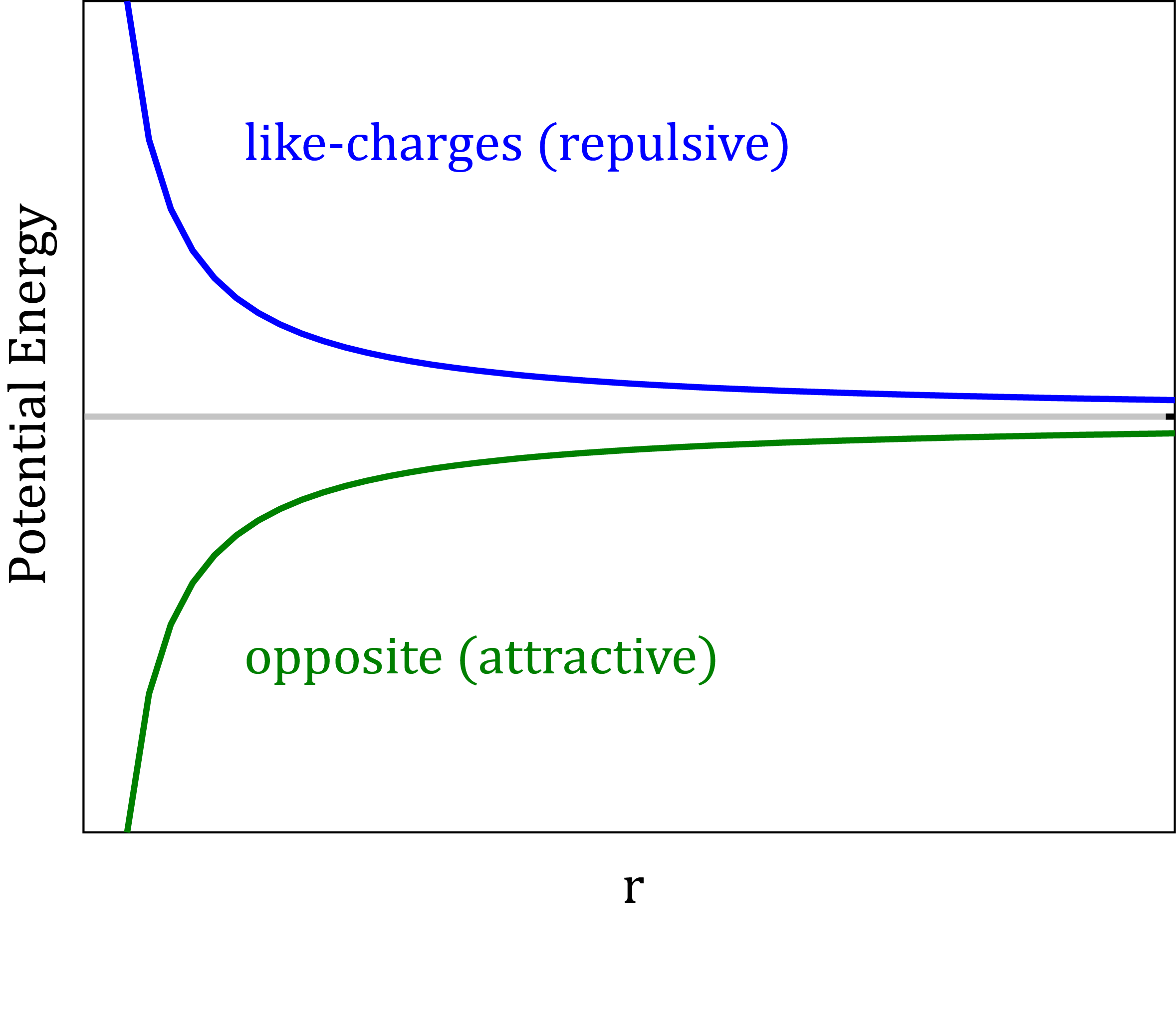
The electrostatic potential
To describe the electrostatic interactions in MD the point charges are assigned to the positions of atomic nuclei. The atomic charges are derived using QM methods with the goal to approximate the electrostatic potential around a molecule. The electrostatic potential is described with the Coulomb’s law:
$V_{Elec}=\frac{q_{i}q_{j}}{4\pi\epsilon_{0}\epsilon_{r}r_{ij}}$
where rij is the distance between the pair of atoms, qi and qj are the charges on the atoms i and j,\(\epsilon_{0}\) is the permittivity of vacuum. and \(\epsilon_{r}\) is the relative permittivity.
- Point charges are assigned to the positions of atomic nuclei to approximate the electrostatic potential around a molecule.
- The Coulomb’s law: $V_{Elec}=\frac{q_{i}q_{j}}{4\pi\epsilon_{0}\epsilon_{r}r_{ij}}$
Short-range and Long-range Interactions
Interactions can be classified as short-range and long-range. In a short-range interaction, the potential decreases faster than r-d, where r is the distance between the particles and d is the dimension. Otherwise the interaction is long-ranged. Accordingly, the Lennard-Jones interaction is short-ranged, while the Coulomb interaction is long-ranged.
- Interaction is short-range if the potential decreases faster than r-3
- The Lennard-Jones interactions are short-ranged, r-6.
- The Coulomb interactions are long-ranged, r-1.
Counting Non-Bonded Interactions
How many non-bonded interactions are in the system with ten Argon atoms? 10, 45, 90, or 200?
Solution
Argon atoms are neutral, so there is no Coulomb interaction. Atoms don’t interact with themselves and the interaction ij is the same as the interaction ji. Thus the total number of pairwise non-bonded interactions is (10x10 - 10)/2 = 45.
Bonded Terms
Bonded terms describe interactions between atoms within molecules. Bonded terms include several types of interactions, such as bond stretching terms, angle bending terms, dihedral or torsional terms, improper dihedrals, and coupling terms.
The bond potential
The bond potential is used to model the interaction of covalently bonded atoms in a molecule. Bond stretch is approximated by a simple harmonic function describing oscillation about an equilibrium bond length r0 with bond constant kb:
- Oscillation about an equilibrium bond length r0 with bond constant kb: $V_{Bond}=k_b(r_{ij}-r_0)^2$
$V_{Bond}=k_b(r_{ij}-r_0)^2$
In a bond, energy oscillates between the kinetic energy of the mass of the atoms and the potential energy stored in the spring connecting them.

This is a fairly poor approximation at extreme bond stretching, but bonds are so stiff that it works well for moderate temperatures. Morse potentials are more accurate, but more expensive to calculate because they involve exponentiation. They are widely used in spectroscopic applications.
- Poor approximation at extreme stretching, but it works well at moderate temperatures.
The angle potential
The angle potential describes the bond bending energy. It is defined for every triplet of bonded atoms. It is also approximated by a harmonic function describing oscillation about an equilibrium angle \(\theta_{0}\) with force constant \(k_\theta\) :
- Oscillation about an equilibrium angle \(\theta_{0}\) with force constant \(k_\theta\): $V_{Angle}=k_\theta(\theta_{ijk}-\theta_0)^2$
$V_{Angle}=k_\theta(\theta_{ijk}-\theta_0)^2$

The force constants for angle potential are about 5 times smaller that for bond stretching.
- The force constants for angle potential are about 5 times smaller that for bond stretching.
The torsion (dihedral) angle potential
The torsion energy is defined for every 4 sequentially bonded atoms. The torsion angle \(\phi\) is the angle of rotation about the covalent bond between the middle two atoms and the potential is given by:
- Defined for every 4 sequentially bonded atoms.
- Sum of any number of periodic functions, n - periodicity, \(\delta\) - phase shift angle.
$V_{Dihed}=k_\phi(1+cos(n\phi-\delta)) + …$
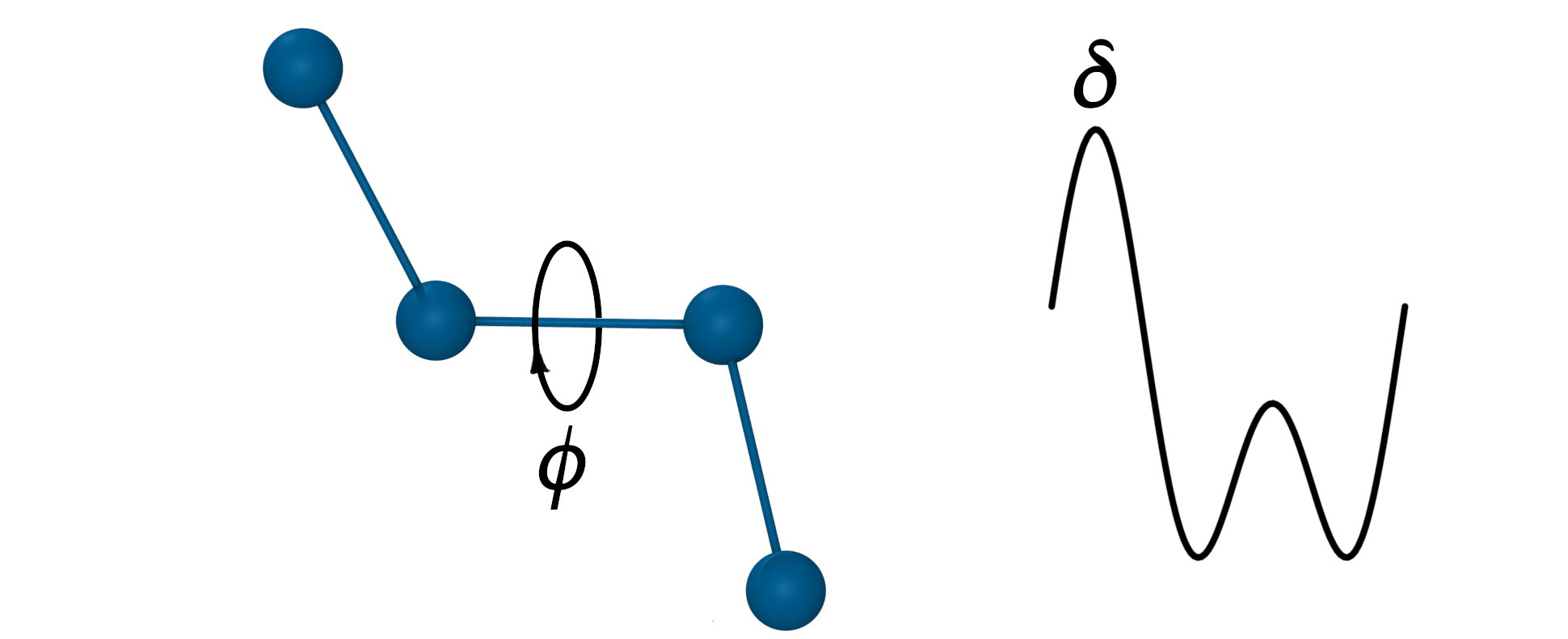
Where the non-negative integer constant n defines periodicity and \(\delta\) is the phase shift angle.
- n represents the number of potential maxima or minima generated in a 360° rotation.

Dihedrals of multiplicity of n=2 and n=3 can be combined to reproduce energy differences of cis/trans and trans/gauche conformations. The example above shows the torsion potential of ethylene glycol.
- Combination of n=2 and n=3 dihedrals used to reproduce cis/trans and trans/gauche energy differences in ethylene glycol
The improper torsion potential
Improper torsion potentials are defined for groups of 4 bonded atoms where the central atom i is connected to the 3 peripheral atoms j,k, and l. Such group can be seen as a pyramid and the improper torsion potential is related to the distance of the central atom from the base of the pyramid. This potential is used mainly to keep molecular structures planar. As there is only one energy minimum the improper torsion term can be given by a harmonic function:
- Also known as ‘out-of-plane bending’
- Defined for a group of 4 bonded atoms where the central atom i is connected to the 3 peripheral atoms j,k, and l.
- Used to enforce planarity.
- Given by a harmonic function: $V_{Improper}=k_\phi(\phi-\phi_0)^2$
$V_{Improper}=k_\phi(\phi-\phi_0)^2$

Where the dihedral angle \(\phi\) is the angle between planes ijk and ijl.
- The dihedral angle \(\phi\) is the angle between planes ijk and ijl.
Coupling Terms
The Urey-Bradley potential
It is known that as a bond angle is decreased, the adjacent bonds stretch to reduce the interaction between the outer atoms of the bonded triplet. This means that there is a coupling between bond length and bond angle. This coupling can be described by the Urey-Bradley potential. The Urey-Bradley term is defined as a (non-covalent) spring between the outer i and k atoms of a bonded triplet ijk. It is approximated by a harmonic function describing oscillation about an equilibrium distance rub with force constant kub:
- Coupling between bond length and bond angle is described by the Urey-Bradley potential.
- The Urey-Bradley term is defined as a spring between the outer atoms of a bonded triplet.
- Approximated by a harmonic function: $V_{UB}=k_{ub}(r_{jk}-r_{ub})^2$
$V_{UB}=k_{ub}(r_{ik}-r_{ub})^2$
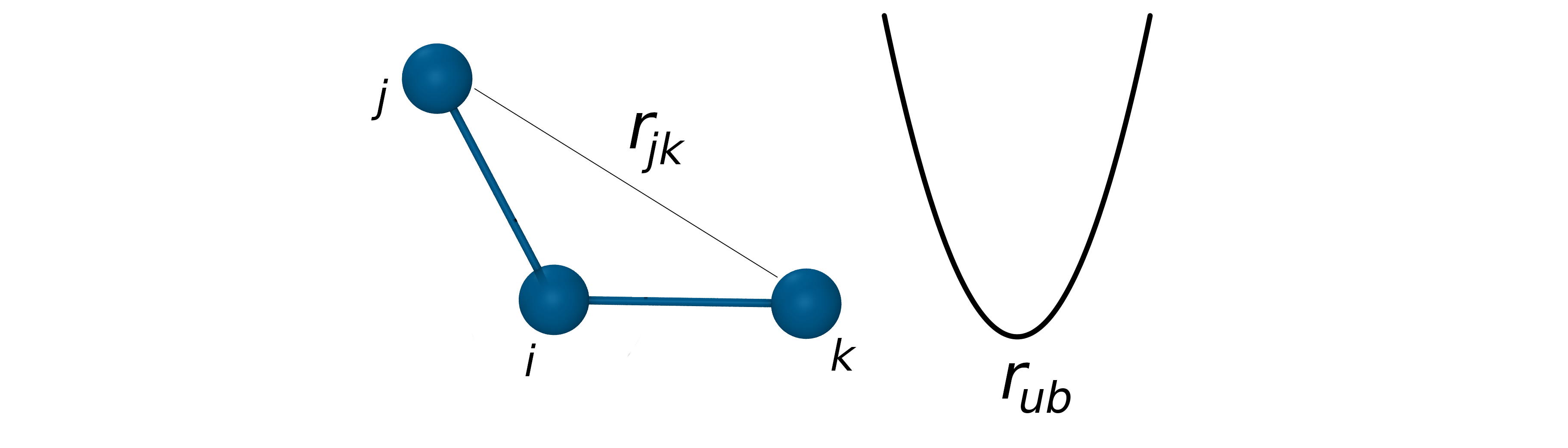
U-B terms are used to improve agreement with vibrational spectra when a harmonic bending term alone would not adequately fit. These phenomena are largely inconsequential for the overall conformational sampling in a typical biomolecular/organic simulation. The Urey-Bradley term is implemented in the CHARMM force fields.
- Improve agreement with vibrational spectra.
- Do not affect overall conformational sampling.
- Implemented in CHARMM and AMOEBA force fields.
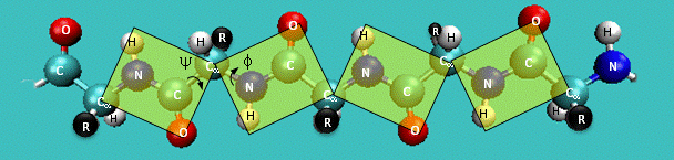
CHARMM CMAP correction potential
A protein can be seen as a series of linked sequences of peptide units which can rotate around phi/psi angles (peptide bond N-C is rigid). These phi/psi angles define the conformation of the backbone.
- Peptide torsion angles: phi, psi, omega.
- A protein can be seen as a series of linked sequences of peptide units which can rotate around phi/psi angles.
- phi/psi angles define the conformation of the backbone.
phi/psi dihedral angle potentials correct for force field deficiencies such as errors in non-bonded interactions, electrostatics, lack of coupling terms, inaccurate combination, etc.
CMAP potential is a correction map to the backbone dihedral energy. It was developed to improve the sampling of backbone conformations. CMAP parameter does not define a continuous function. it is a grid of energy correction factors defined for each pair of phi/psi angles typically tabulated with 15 degree increments.
- phi/psi dihedral angle potentials correct for force field deficiencies such as errors in non-bonded interactions, electrostatics, lack of coupling terms, inaccurate combination, etc.
- CMAP potential was developed to improve the sampling of backbone conformations.
- CMAP parameter does not define a continuous function.
- it is a grid of energy correction factors defined for each pair of phi/psi angles typically tabulated with 15 degree increments.
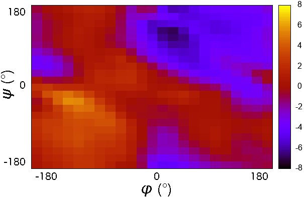
The grid of energy correction factors is constructed using QM data for every combination of \(\phi/\psi\) dihedral angles of the peptide backbone and further optimized using empirical data.
CMAP potential was initially applied to improve CHARMM22 force field. CMAP corrections were later implemented in AMBER force fields ff99IDPs (force field for intrinsically disordered proteins), ff12SB-cMAP (force field for implicit-solvent simulations), and ff19SB.
Energy scale of potential terms
| \(k_BT\) at 298 K | ~ 0.593 | \(\frac{kcal}{mol}\) |
| Bond vibrations | ~ 100 ‐ 500 | \(\frac{kcal}{mol \cdot \unicode{x212B}^2}\) |
| Bond angle bending | ~ 10 - 50 | \(\frac{kcal}{mol \cdot deg^2}\) |
| Dihedral rotations | ~ 0 - 2.5 | \(\frac{kcal}{mol \cdot deg^2}\) |
| van der Waals | ~ 0.5 | \(\frac{kcal}{mol}\) |
| Hydrogen bonds | ~ 0.5 - 1.0 | \(\frac{kcal}{mol}\) |
| Salt bridges | ~ 1.2 - 2.5 | \(\frac{kcal}{mol}\) |
Exclusions from Non-Bonded Interactions
Pairs of atoms connected by chemical bonds are normally excluded from computation of non-bonded interactions because bonded energy terms replace non-bonded interactions. In biomolecular force fields all pairs of connected atoms separated by up to 2 bonds (1-2 and 1-3 pairs) are excluded from non-bonded interactions.
Computation of the non-bonded interaction between 1-4 pairs depends on the specific force field. Some force fields exclude VDW interactions and scale down electrostatic (AMBER) while others may modify both or use electrostatic as is.
- In pairs of atoms connected by chemical bonds bonded energy terms replace non-bonded interactions.
- All pairs of connected atoms separated by up to 2 bonds (1-2 and 1-3 pairs) are excluded from non-bonded interactions. It is assumed that they are properly described with bond and angle potentials.

The 1-4 interaction turns out to be an intermediate case where both bonded and non-bonded interactions are required for a reasonable description. Due to the short distance between the 1–4 atoms full strength non-bonded interactions are too strong, and in most cases lack fine details of local internal conformational degrees of freedom. To address this problem in many cases a compromise is made to treat this particular pair partially as a bonded and partially as a non-bonded interaction.
Non-bonded interactions between 1-4 pairs depends on the specific force field. Some force fields exclude VDW interactions and scale down electrostatic (AMBER) while others may modify both or use electrostatic as is.
- 1-4 interaction represents a special case where both bonded and non-bonded interactions are required for a reasonable description. However, due to the short distance between the 1–4 atoms full strength non-bonded interactions are too strong and must be scaled down.
- Non-bonded interaction between 1-4 pairs depends on the specific force field.
- Some force fields exclude VDW interactions and scale down electrostatic (AMBER) while others may modify both or use electrostatic as is.
What Information Can MD Simulations Provide?
With the help of MD it is possible to model phenomena that cannot be studied experimentally. For example
- Understand atomistic details of conformational changes, protein unfolding, interactions between proteins and drugs
- Study thermodynamics properties (free energies, binding energies)
- Study biological processes such as (enzyme catalysis, protein complex assembly, protein or RNA folding, etc).
For more examples of the types of information MD simulations can provide read the review article: Molecular Dynamics Simulation for All.
Specifying Exclusions
GROMACS
The exclusions are generated by grompp as specified in the [moleculetype] section of the molecular topology .top file:
[ moleculetype ]
; name  nrexcl
Urea         3
...
[ exclusions ]
;  ai    aj
   1     2
   1     3
   1     4
In the example above non-bonded interactions between atoms that are no farther than 3 bonds are excluded (nrexcl=3). Extra exclusions may be added explicitly in the [exclusions] section.
The scaling factors for 1-4 pairs, fudgeLJ and fudgeQQ, are specified in the [defaults] section of the forcefield.itp file. While fudgeLJ is used only when gen-pairs is set to ‘yes’, fudgeQQ is always used.
[ defaults ]
; nbfunc        comb-rule       gen-pairs       fudgeLJ fudgeQQ
1               2               yes             0.5     0.8333
NAMD
Which pairs of bonded atoms should be excluded is specified by the exclude parameter.
Acceptable values: none, 1-2, 1-3, 1-4, or scaled1-4exclude scaled1-4 1-4scaling 0.83 scnb 2.0If scaled1-4 is set, the electrostatic interactions for 1-4 pairs are multiplied by a constant factor specified by the 1-4scaling parameter. The LJ interactions for 1-4 pairs are divided by scnb.
Key Points
Molecular dynamics simulates atomic positions in time using forces acting between atoms
The forces in molecular dynamics are approximated by simple empirical functions